Understanding Factor Behavior: Interpreting Main Effects and Interaction Plots

1. Visualizing Individual Factor Effects: Main Effects Plots

After identifying significant factors with ANOVA, the first step is to visualize their individual impact using a Main Effects Plot. This simple line graph shows the average response value at each level of a single factor.

By examining the plot, you can quickly answer two critical questions:

1. What is the magnitude of the effect? The steeper the slope of the line connecting the points, the stronger the effect. A nearly horizontal line indicates the factor has little to no effect on the response.
2. What is the direction of the effect? The plot shows whether the response increases or decreases as you move from the low level to the high level of the factor.

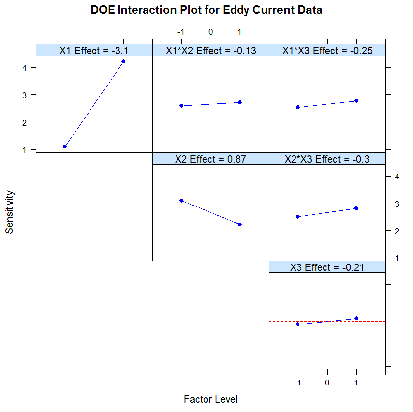
For a clear, practical guide on what these plots tell you, let's look at an example from a juice bottling plant.

As the article demonstrates, you can quickly determine that to minimize negative bias, you should target lower dry matter content and larger particle sizes, while speed appears to have no significant influence. This is the power of a main effects plot: turning data into direction.

2. Uncovering Hidden Relationships: Interaction Plots

In the previous lesson, we emphasized a critical rule: if an interaction effect (e.g., A*B) is significant, you must interpret it before considering the main effects (A and B) individually. Interaction plots are the tool that makes this possible.

An interaction occurs when the effect of one factor on the response is different at different levels of another factor. An interaction plot visualizes this by plotting the average response for every combination of factor levels.

The key to interpretation lies in the lines on the plot:

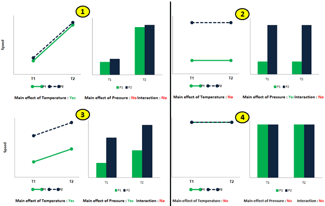
• Parallel Lines: The effect of one factor is the same regardless of the other factor's level. This indicates no interaction.
• Non-Parallel Lines: The lines converge or diverge. This shows that the effect of one factor is dependent on the level of the other. This indicates an interaction.
• Crossing Lines: This is a strong, or "antagonistic," interaction. The effect of one factor completely reverses depending on the level of the other.

To build a strong visual intuition for this, please watch the following videos. They break down these concepts clearly with graphical examples.

To summarize the patterns you just saw:

3. A Practical Manufacturing Case Study: Optimizing Tool Life

Now, let's apply this to a realistic scenario. As an Industrial Engineer in manufacturing, optimizing tool life is a common and high-impact project.

Imagine you've completed a $2^3$ factorial experiment to study the effects of Cutting Speed (A), Tool Geometry (B), and Cutting Angle (C) on the life of a machine tool.

From the previous lesson, you ran the ANOVA and found the following significant effects (p < 0.05):

• Factor B (Tool Geometry)
• Factor C (Cutting Angle)
• The AC Interaction (Cutting Speed * Cutting Angle)

Our task is to interpret the plots to recommend the optimal machine settings for the longest tool life.

Let's break down the interpretation, following the rules we've established:

1. Analyze the Significant Interaction First: The ANOVA told us the AC interaction is significant. The plot shows two non-parallel lines, confirming this visually. Our goal is to maximize tool life, so we look for the highest point on the graph. This occurs when Cutting Angle (C) is at its high level (+1) and Cutting Speed (A) is at its low level (-1). We can lock in these two settings.

2. Analyze Remaining Significant Main Effects: The other significant factor was Tool Geometry (B). It was not involved in any significant interactions, so we can interpret its main effect directly. The ANOVA table shows its effect estimate is positive (5.67). This means moving from the low to the high level of B increases tool life. Therefore, we should set Tool Geometry (B) at its high level (+1).

3. Formulate the Recommendation: By combining these insights, we arrive at the optimal conditions for maximizing tool life:

   • Cutting Speed (A): Low Level
   • Tool Geometry (B): High Level
   • Cutting Angle (C): High Level

This step-by-step process, starting with the ANOVA results and using the plots for interpretation, is fundamental to the Analyze phase of any DOE project.

Conclusion

In this lesson, you learned how to translate the statistical output of an ANOVA into practical, visual insights using main effects and interaction plots. These graphs are not just pictures; they are the tools you use to understand the behavior of your process and communicate your findings to stakeholders.

Key Takeaways:

• Main Effects Plots show the average impact of a single factor on the response. The slope indicates the strength and direction of the effect.
• Interaction Plots reveal how factors work together. The golden rule is that non-parallel lines indicate an interaction.
• Always interpret significant interactions first. A significant interaction plot dictates the optimal settings for the factors involved, overriding their individual main effects.

Preview of the Next Lesson:

We have now identified the vital few factors, understood their behavior, and even recommended the best combination of levels tested in our experiment. But what if the true optimal setting lies between the levels we tested? For example, we tested temperatures of 100°C and 150°C, but what if the peak performance is actually at 127°C?

In our next lesson, we will introduce Response Surface Methodology (RSM). This advanced DOE technique allows us to model curvature in the response and use that model to find the true optimal settings for our process, helping us climb to the very peak of the performance mountain.