MLE for Gaussian Parameters

The Goal: Finding the "Best" Gaussian

Imagine you have a set of data points, and you hypothesize they were drawn from some Gaussian distribution. The problem is, you don't know which one. A Gaussian distribution is defined by two parameters: its mean ($\mu$), which sets its center, and its variance (${\sigma }^2$), which controls its spread. Our task is to find the specific values of $\mu$ and ${\sigma }^2$ that define the single Gaussian curve that best fits our data.

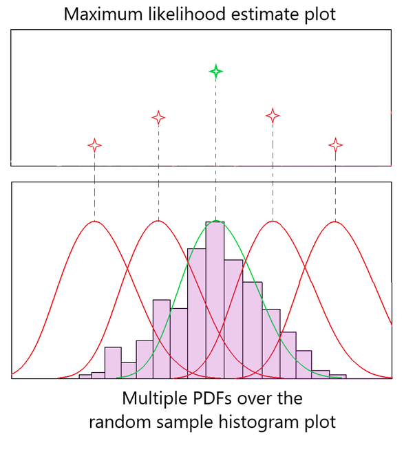
The principle of maximum likelihood gives us a precise way to define "best fit." We want to find the parameters that maximize the likelihood function. The image below provides the intuition for this. Given a histogram of data, we can imagine overlaying many different Gaussian probability density functions (PDFs). MLE is the process of finding the one curve (the green one) for which the likelihood of observing our data is at its peak.

The MLE Derivation: Recipe and Walkthrough

To find the parameters that maximize the likelihood function, we follow a standard four-step mathematical recipe:

1. Write the Likelihood Function: Assume the data points are independent and identically distributed (IID), and write the joint probability of the entire dataset as a function of the parameters. This is the product of the individual probabilities.
2. Take the Log-Likelihood: Take the natural logarithm of the likelihood function. This turns the product into a sum, which is much easier to differentiate. Since the logarithm is a monotonically increasing function, maximizing the log-likelihood is equivalent to maximizing the original likelihood.
3. Take Partial Derivatives: Calculate the partial derivative of the log-likelihood function with respect to each parameter you want to estimate (in our case, $\mu$ and ${\sigma }^2$).
4. Solve: Set the derivatives equal to zero and solve the resulting system of equations. The solutions will be your maximum likelihood estimates.

The following video from StatQuest provides an exceptionally clear, step-by-step walkthrough of this entire process. While it's detailed, we'll focus on the core mathematical segments.

Formalizing the Derivation

The StatQuest video provided a fantastic intuition and visual guide. Now, let's solidify that understanding by laying out the mathematical steps formally. This will serve as a concise reference for the derivation. The following reading provides a dense, clear summary of these steps.

To summarize the key results from the derivation, given a dataset of $n$ samples $x_1,x_2,\dots ,x_n$:

1. Log-Likelihood Function:
   The log-likelihood function for a Gaussian distribution simplifies to:

   $$\mathcal{L}(\mu ,{\sigma }^2)=-\frac{n}{2}\log (2\pi )-\frac{n}{2}\log ({\sigma }^2)-\frac{1}{2{\sigma }^2}\sum _{i=1}^n(x_i-\mu {)}^2$$

2. MLE for the Mean ($\mu$):
   By taking the partial derivative $\frac{\partial \mathcal{L}}{\partial \mu }$, setting it to zero, and solving, we find:

   $${\hat{\mu }}_{\text{MLE}}=\frac{1}{n}\sum _{i=1}^n{x}_i$$

   This is simply the sample mean of the data.

3. MLE for the Variance (${\sigma }^2$):
   By taking the partial derivative $\frac{\partial \mathcal{L}}{\partial {\sigma }^2}$, setting it to zero, and solving, we get:

   $${\hat{\sigma }}_{\text{MLE}}^2=\frac{1}{n}\sum _{i=1}^n(x_i-\hat{\mu }{)}^2$$

   This is the sample variance of the data, calculated using the MLE estimate for the mean, $\hat{\mu }$.

These results are powerful because they are so intuitive. The "most likely" Gaussian distribution to have generated your data is the one centered at your data's average, with a variance that matches your data's average squared distance from that center. MLE gives us a formal, rigorous proof for using these familiar estimators.

It's worth noting a subtle but important point for your future studies. The MLE for variance, ${\hat{\sigma }}^2$, is known as a biased estimator. In many statistical packages, you'll find that the sample variance is calculated with a denominator of $n-1$ instead of $n$. That version is an unbiased estimator. While they are numerically very similar for large datasets, this distinction is theoretically important and something we may revisit later.

Conclusion

In this lesson, you have walked through the complete mathematical derivation of the Maximum Likelihood Estimators for the parameters of a Gaussian distribution. You saw how a standard, multi-step process involving the log-likelihood function and partial derivatives leads to the intuitive result that the sample mean and sample variance are the MLEs for $\mu$ and ${\sigma }^2$. This process serves as a template for deriving estimators for many other probabilistic models in machine learning.

In our next lesson, we will build directly on this foundation. We will move to Maximum A Posteriori (MAP) estimation, applying it to a linear regression problem. This will bring us back to the Bayesian perspective by incorporating a prior, and you will see a fascinating connection between MAP and the regularization techniques you are already familiar with.