MAP Estimation in Linear Regression

From Likelihood to Posterior: The Bayesian Shift

In MLE, our objective was to maximize the likelihood function, $P(D|\theta )$, where $D$ is the data and $\theta$ is the parameter set. The question was, "What parameters make our data most probable?"

MAP estimation takes this one step further by asking, "Given our data, what parameters are most probable?" This corresponds to maximizing the posterior probability, $P(\theta |D)$. To do this, we use Bayes' theorem:

The key insight is that MAP incorporates a prior distribution, $P(\theta )$, which represents our belief about the parameters before we see any data. The likelihood, $P(D|\theta )$, then updates this prior belief to form the posterior. The term in the denominator, $P(D)$, is the probability of the data itself. Since it doesn't depend on $\theta$, we can treat it as a constant normalizer and ignore it for the purpose of maximization.

This leads to the core objective of MAP:

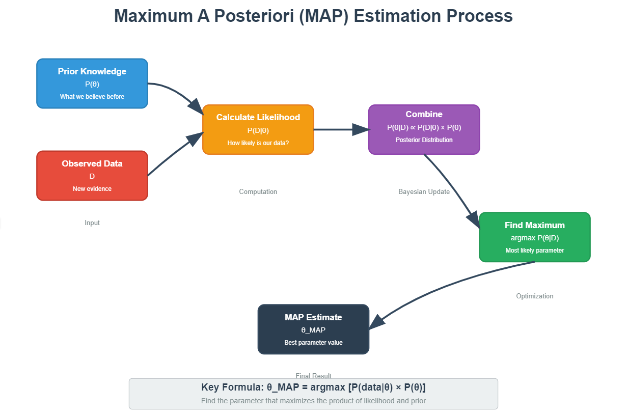
The process is visually summarized in the diagram below. We start with our prior knowledge and observed data, combine them via Bayesian update to get the posterior distribution, and then find the parameter value that maximizes this posterior.

The Log-Posterior and the Role of the Prior

Just as with MLE, working with products of probabilities is cumbersome. We can simplify the objective by taking the logarithm. Since the logarithm is a monotonically increasing function, maximizing the posterior is equivalent to maximizing the log-posterior:

Compare this to the log-likelihood objective from our last lesson:

The only difference is the addition of the log-prior term, $\log (P(\theta ))$. This term acts as a "guide" or a penalty, pulling the final estimate towards regions of the parameter space that we believed were more likely to begin with.

For a more formal breakdown of this formulation, you can consult the following lecture notes.

MAP for Linear Regression: The Emergence of Regularization

Now for the main event. Let's apply this framework to a linear regression model. You'll see how choosing a specific prior for our regression weights naturally leads to the L2 regularization you know as Ridge Regression. This connection is one of the most elegant results in introductory machine learning theory.

The following video from the channel ritvikmath provides an outstanding explanation of this entire process. It begins with a review of regularized regression and then masterfully builds the Bayesian argument that leads to the same place.

Unpacking the Derivation

Let's summarize the beautiful result from the video.

1. Likelihood: We assume the standard linear regression model $y_i={\mathbf{w}}^T{\mathbf{x}}_i+{ϵ}_i$, with Gaussian noise ${ϵ}_i\sim \mathcal{N}(0,{\sigma }^2)$. This gives us a Gaussian likelihood $P(D|\mathbf{w})$. Maximizing the log of this likelihood alone leads to the ordinary least squares (OLS) solution, which is the MLE for linear regression. The objective is to minimize the Residual Sum of Squares (RSS):

   $${\mathbf{w}}_{\text{MLE}}=\underset{\mathbf{w}}{\mathrm{argmin}}\sum _{i=1}^n(y_i-{\mathbf{w}}^T{\mathbf{x}}_i{)}^2$$

2. Prior: We place a Gaussian prior on our weights, assuming they are centered at zero: $\mathbf{w}\sim \mathcal{N}(0,{\tau }^{2}I)$. This expresses our prior belief that smaller weights are more likely than larger ones. The log of this prior is:

   $$\log P(\mathbf{w})\propto -\frac{1}{2{\tau }^2}\sum _{j=1}^p{w}_j^2=-\frac{1}{2{\tau }^2}\Vert \mathbf{w}{\Vert }_2^2$$

3. Posterior: Combining the log-likelihood and the log-prior, the MAP objective becomes minimizing the negative log-posterior:

   $${\mathbf{w}}_{\text{MAP}}=\underset{\mathbf{w}}{\mathrm{argmin}}\left(\sum _{i=1}^n(y_i-{\mathbf{w}}^T{\mathbf{x}}_i{)}^2+\frac{{\sigma }^2}{{\tau }^2}\Vert \mathbf{w}{\Vert }_2^2\right)$$

This is exactly the objective function for Ridge Regression, where the regularization parameter $\lambda$ is equal to the ratio of the noise variance to the prior variance, $\lambda ={\sigma }^2/{\tau }^2$.

This gives us a powerful Bayesian interpretation of L2 regularization: it is equivalent to performing MAP estimation with a zero-mean Gaussian prior on the model weights. The strength of the regularization, $\lambda$, is determined by how strongly we believe the weights should be close to zero (a small prior variance ${\tau }^2$) relative to the amount of noise in the data (${\sigma }^2$).

The following article provides a practical code demonstration, showing how sklearn.linear_model.Ridge is, in fact, an implementation of this MAP estimate.

As the video and other resources hint, choosing a different prior leads to a different form of regularization. For instance, if we had chosen a Laplace prior on the weights, which is more "peaked" at zero, the MAP estimate would have corresponded to Lasso (L1) regression.

Conclusion

In this lesson, you have connected several fundamental concepts. You've learned that Maximum A Posteriori (MAP) estimation extends MLE by incorporating prior beliefs about parameters. Most importantly, you have seen the direct mathematical link between MAP estimation for linear regression and Ridge (L2) regularization. A Gaussian prior on the weights is not just an arbitrary choice; it is the Bayesian justification for the L2 penalty term that you have likely used many times in practice. This insight elevates regularization from a mere "trick" to prevent overfitting to a principled application of Bayesian inference.

In our next lesson, we will dive deeper into the practicalities of Bayesian updates by exploring the concept of conjugate priors. You will learn how choosing a specific mathematical pairing of a prior and a likelihood can make calculating the posterior distribution surprisingly simple. We will demonstrate this by deriving the posterior for a classic Beta-Binomial model.