Beta-Binomial Conjugacy

In our last lesson, we explored Maximum A Posteriori (MAP) estimation and discovered a fascinating link between Bayesian priors and regularization. By adding a Gaussian prior to the weights of a linear regression model, we derived the exact objective function for Ridge regression. This showed how a prior belief can be used to guide a model, moving beyond just maximizing the likelihood of the data.

Today, we'll delve deeper into the interplay between priors and likelihoods. While MAP estimation focuses on finding the single most probable parameter value (the posterior's peak), we often want to understand the entire posterior distribution. Calculating this can be mathematically intensive. This lesson introduces a powerful shortcut: conjugate priors. Your goal is to explain the concept of conjugate priors by deriving the posterior for a Beta-Binomial model. This will provide you with a cornerstone concept in Bayesian modeling, showcasing how a clever choice of prior can make Bayesian updates both computationally simple and wonderfully intuitive.

The Problem: Modeling a Probability

Imagine a simple scenario: you're trying to determine the underlying probability, let's call it $p$ , of an event with two outcomes. This could be the probability of a coin landing heads, a user clicking an advertisement, or a manufactured part passing a quality check. Since $p$ is a probability, its value must be between 0 and 1.

Our Bayesian framework requires two key components:

A Likelihood Function: This describes the probability of observing our data given a specific value of $p$ . If we conduct $n$ independent trials and observe $k$ "successes," the Binomial distribution is the natural choice to model this process. The likelihood function is proportional to $p^{k} (1 - p)^{n - k}$ .
A Prior Distribution: This captures our beliefs about $p$ before seeing any data. We need a probability distribution defined on the interval [0, 1].

The following video introduces this exact problem using a memorable story about skipping rocks. It will help you set up the likelihood and motivate the choice of a prior.

Conjugate Priors : Data Science Basics

This video from the channel ritvikmath, titled "Conjugate Priors," provides an excellent, story-driven introduction to the topic.

First, watch the setup of the problem from the beginning. This will establish the Binomial distribution as the correct likelihood for modeling the number of successes in a series of trials. Next, watch the introduction to the Beta distribution as a natural choice for the prior from this section. Pay attention to the interpretation of its hyperparameters, \alpha and \beta.

The Prior: Shaping Beliefs with the Beta Distribution

As the video explained, the Beta distribution is an ideal choice for a prior on a probability parameter. Its probability density function (PDF) is given by:

f (p; α, β) = \frac{p ^{α - 1} ( 1 - p ) ^{β - 1}}{B ( α , β )}

where $B (α, β)$ is a normalizing constant ensuring the area under the curve is 1.

The key lies in the hyperparameters $α$ and $β$ . They shape our prior belief and are often interpreted as "pseudo-counts" from past experience:

$α - 1$ represents the number of prior "successes."
$β - 1$ represents the number of prior "failures."

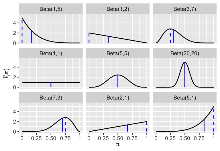
By adjusting $α$ and $β$ , we can model a wide range of beliefs.

If $α = β = 1$ , the distribution is uniform—we believe all values of $p$ are equally likely.
If $α > β$ , the distribution is skewed towards 1, indicating a prior belief that successes are more likely.
If $α$ and $β$ are large, the distribution becomes narrow and sharply peaked, indicating a strong, confident prior belief.

The image below shows how different settings of $α$ and $β$ create a variety of distribution shapes.

A grid of nine plots showing the probability density function of the Beta distribution for various $\alpha$ and $\beta$ parameters. This illustrates how the hyperparameters control the shape, mean (solid blue line), and mode (dashed blue line) of the distribution, making it a flexible choice for a prior.

For a more detailed look at the properties of the Beta distribution, the following reading is highly recommended.

Chapter 3 The Beta-Binomial Bayesian Model

This chapter from the online book Bayes Rules! provides a thorough and accessible walkthrough of the Beta-Binomial model.

Focus on Section 3.1, specifically the part on Beta foundations. Then, carefully read the explanation of how the mean, mode, and variance are calculated from the hyperparameters in the paragraphs starting from "The mean (or 'expected value')".

The "Magic": Deriving the Posterior

Now we combine our Beta prior with our Binomial likelihood using Bayes' theorem to find the posterior distribution. Recall that the posterior is proportional to the product of the likelihood and the prior:

P (p ∣ data) \propto P (data ∣ p) \times P (p)

Let's substitute the functional forms we've chosen. Let our data consist of $k$ successes in $n$ trials.

Posterior P (p ∣ k, n) \propto Likelihood (Binomial kernel) p^{k} (1 - p)^{n - k} \times Prior (Beta kernel) p^{α - 1} (1 - p)^{β - 1}

We can ignore the normalizing constants $(k n)$ from the likelihood and $B (α, β)$ from the prior, as they don't depend on $p$ . Now, we simply combine the terms by adding the exponents:

P (p ∣ k, n) \propto p^{(k + α) - 1} \cdot (1 - p)^{(n - k + β) - 1}

Look closely at this result. This is the kernel of another Beta distribution! This means our posterior distribution is:

P (p ∣ k, n) \sim Beta (α^{'} = α + k, β^{'} = β + n - k)

This elegant result is the heart of conjugacy. We started with a Beta prior, and after updating it with Binomial data, we ended up with another Beta distribution. The following handwritten derivation summarizes this process neatly.

This image shows the step-by-step mathematical derivation for the Beta-Binomial model. It starts with Bayes' theorem, substitutes the Binomial likelihood and Beta prior, combines the terms, and shows that the resulting posterior is a Beta distribution with updated parameters.

The next segment of the ritvikmath video walks through this derivation with excellent commentary.

Conjugate Priors : Data Science Basics

Let's return to the "Conjugate Priors" video to see this derivation in action.

Watch from this section, where the presenter applies Bayes' theorem. Follow the algebraic simplification as he combines the terms from the prior and the likelihood. Then, watch the conclusion of the derivation, where he reveals that the posterior is also a Beta distribution.

The Definition and Importance of Conjugacy

We have just demonstrated a case of conjugacy. A prior distribution is said to be a conjugate prior for a given likelihood function if the resulting posterior distribution belongs to the same family of distributions as the prior.

In our case:

The Beta distribution is the conjugate prior for the...
Binomial (or Bernoulli) likelihood function.
The posterior is also a Beta distribution.

Why is this so important?

Computational Simplicity: The update rule is trivial. Instead of performing complex integration to find the posterior, we just update the parameters: $α_{n e w} = α_{o l d} + k$ and $β_{n e w} = β_{o l d} + (n - k)$ .
Interpretability: This is arguably the most powerful benefit. The update tells a clear story. Our prior belief was quantified by $α$ pseudo-successes and $β$ pseudo-failures. After observing $k$ real successes and $n - k$ real failures, our posterior belief is simply the sum of our prior and observed counts. This makes the process of Bayesian belief updating transparent and easy to reason about.

The final part of the video explains this significance beautifully.

Conjugate Priors : Data Science Basics

This last segment of the "Conjugate Priors" video explains why this concept is so fundamental.

Watch from this explanation of the parameter update rule. The key insight is how the posterior parameters literally incorporate the observed data into the prior's pseudo-counts. Finally, watch the summary from "why we care," which correctly emphasizes the value of interpretability.

Conclusion

In this lesson, you have learned about one of the most elegant and practical concepts in Bayesian statistics. By pairing a Binomial likelihood with a Beta prior, we found that the posterior distribution is also a Beta distribution. This special relationship, known as conjugacy, simplifies Bayesian inference tremendously.

Key Takeaways:

A conjugate prior is a prior distribution that, when combined with a specific likelihood, yields a posterior distribution from the same family.
The Beta distribution is the conjugate prior for the Binomial likelihood.
The update rule for the Beta-Binomial model is simple and intuitive: the new hyperparameters are found by adding the observed number of successes and failures to the prior's hyperparameters ( $α^{'} = α + k$ , $β^{'} = β + n - k$ ).
The primary benefits of using conjugate priors are analytical tractability and, more importantly, the interpretability of the belief-updating process.

So far, we have explored parameter estimation from frequentist (MLE) and Bayesian (MAP, Conjugate Priors) perspectives. In the next lesson, we will apply this probabilistic foundation to a classic machine learning task: classification. You will learn to implement the training logic for a Gaussian Naive Bayes classifier from scratch, combining probability theory with algorithmic thinking.

Recommended resources

The Problem: Modeling a Probability

The Prior: Shaping Beliefs with the Beta Distribution

The "Magic": Deriving the Posterior

The Definition and Importance of Conjugacy

Conclusion