Gaussian Naive Bayes Training From Scratch

From Bayes' Theorem to a "Naive" Classifier

At its core, the Naive Bayes classifier uses Bayes' theorem to determine the most probable class for a given data point. For a data point with features $\mathbf{x}=(x_1,x_2,\dots ,x_n)$ and a set of possible classes $C_k$, we want to find the class that maximizes the posterior probability $P(C_k|\mathbf{x})$.

According to Bayes' theorem:

Since $P(\mathbf{x})$ is the same for all classes, we can ignore it for comparison and focus on the numerator:

The "naive" part of the algorithm is a crucial simplifying assumption: it assumes that all features $x_i$ are conditionally independent given the class $C_k$. This allows us to break down the complex likelihood term into a simple product:

This assumption is rarely true in reality (for example, in a medical dataset, height and weight are not independent), but it makes the model computationally efficient and surprisingly effective.

The following video provides an excellent mathematical walkthrough of this entire framework, from Bayes' theorem to the naive assumption and the introduction of the Gaussian model.

The "Gaussian" Assumption and the "Training" Process

The classifier we are building is specifically a Gaussian Naive Bayes. This means we assume that for each class $C_k$, the values of any continuous feature $x_i$ are distributed according to a Gaussian (Normal) distribution.

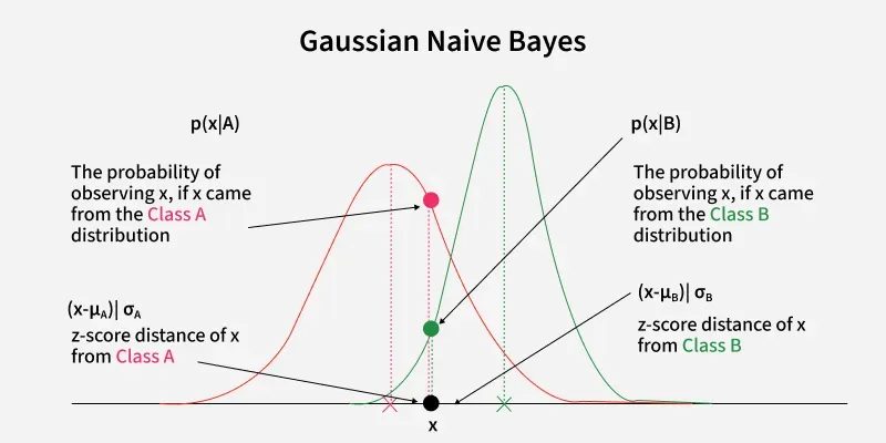
Therefore, to model the likelihood $P(x_i|C_k)$, we just need the parameters of the corresponding Gaussian distribution: its mean ${\mu }_{i,k}$ and its variance ${\sigma }_{i,k}^2$.

This brings us to the "training" phase. For a Naive Bayes classifier, training is not an iterative optimization process like gradient descent. Instead, it is a straightforward process of calculating and storing the parameters that define our model directly from the training data. These parameters are:

1. Class Priors $P(C_k)$: The overall probability of each class.
2. Class-conditional Means ${\mu }_{i,k}$: The mean of each feature $i$ for each class $k$.
3. Class-conditional Variances ${\sigma }_{i,k}^2$: The variance of each feature $i$ for each class $k$.

How do we estimate these? We use the same principle we saw in our second lesson: Maximum Likelihood Estimation (MLE).

As you can see from the reading, the MLE estimates are exactly what you would intuitively expect:

• The prior $P(C_k)$ is the frequency of class $C_k$ in the dataset:
  $\hat{P}(C_k)=\frac{\text{Number of samples in class }k}{\text{Total number of samples}}$
• The mean ${\hat{\mu }}_{i,k}$ is simply the average of feature $i$ for all samples that belong to class $k$.
• The variance ${\hat{\sigma }}_{i,k}^2$ is the variance of feature $i$ for all samples that belong to class $k$.

This is the entire training logic. We will now implement this in Python.

Implementing the Training Logic from Scratch

We will structure our implementation as a Python class with a fit method, similar to the convention used in scikit-learn. The fit method will take the training data X and labels y and perform the three calculations we just discussed, storing the results in the object's attributes.

The following reading provides a clear, step-by-step implementation. We will focus only on the training logic today.

Let's break down the logic from the article.

1. Initialization: The fit method starts by identifying the unique classes and getting the number of samples and features. It then prepares empty NumPy arrays (self.means, self.variances, self.priors) to store the parameters we will calculate.

2. Iterating Over Classes: The core of the method is a loop that iterates through each unique class c.

3. Calculating Parameters for each Class: Inside the loop, for each class c:

   • It first isolates all the data points X_c that belong to that class.
   • It calculates the prior probability for class c by dividing the number of samples in X_c by the total number of samples.
   • It calculates the mean of each feature for the data X_c (using .mean(axis=0)). This gives us the vector of means ${\mu }_{\cdot ,c}$.
   • It calculates the variance of each feature for the data X_c (using .var(axis=0)). This gives us the vector of variances ${\sigma }_{\cdot ,c}^2$.

After the loop finishes, the self.priors, self.means, and self.variances attributes are fully populated. The "training" is complete!

Here is a Python class stub that encapsulates this logic, closely following the structure from the resources.

import numpy as np

class NaiveBayes:
    def fit(self, X, y):
        n_samples, n_features = X.shape
        self._classes = np.unique(y)
        n_classes = len(self._classes)




        # 1. Initialize arrays for parameters
        self._means = np.zeros((n_classes, n_features), dtype=np.float64)
        self._variances = np.zeros((n_classes, n_features), dtype=np.float64)
        self._priors = np.zeros(n_classes, dtype=np.float64)




        # 2. Loop through each class
        for idx, c in enumerate(self._classes):



            # Get all samples for the current class
            X_c = X[y == c]




            # 3. Calculate and store parameters
            self._means[idx, :] = X_c.mean(axis=0)
            self._variances[idx, :] = X_c.var(axis=0)
            self._priors[idx] = X_c.shape[0] / float(n_samples)

This fit method perfectly executes the training logic required by our learning outcome. It computes all the necessary statistical properties from the training data and saves them. These stored parameters now represent our "trained model."

Conclusion

In this lesson, you have learned how to construct the training logic for a Gaussian Naive Bayes classifier. We've seen how this algorithm, despite its "naive" assumption of feature independence, provides a powerful and efficient way to perform classification by modeling feature likelihoods with Gaussian distributions.

Key Takeaways:

• Naive Bayes uses Bayes' theorem to find the most probable class for a new data point.
• The "naive" assumption is that all features are conditionally independent given the class, which simplifies the likelihood calculation to a product of individual probabilities.
• The "Gaussian" part means we model the probability of each continuous feature within a class, $P(x_i|C_k)$, using a Gaussian distribution.
• "Training" a GNB classifier means calculating and storing three sets of parameters from the data: the prior probability of each class, and the mean and variance of each feature for each class.
• These parameters are estimated using Maximum Likelihood Estimation, connecting directly back to our earlier lessons on parameter estimation.

In our next lesson, we will complete our classifier by implementing the prediction logic. We will use the priors, means, and variances we've just learned to calculate the posterior probability for new, unseen data points and make our final classification.