Implementing Gaussian Naive Bayes from Scratch

The Heart of Prediction: Calculating Posterior Probabilities

With our trained model, the task of prediction for a new data point $\mathbf{x}=(x_1,x_2,\dots ,x_n)$ is to find the class $C_k$ that is most probable given the data. This is known as finding the Maximum A Posteriori (MAP) estimate. We want to find the class $k$ that maximizes the posterior probability $P(C_k|\mathbf{x})$.

From our previous lesson, we know that Bayes' theorem gives us:

Thanks to the "naive" independence assumption, the likelihood term simplifies to a product:

And because this is a "Gaussian" Naive Bayes, we calculate each $P(x_i|C_k)$ using the probability density function (PDF) of a Gaussian distribution, whose parameters (${\mu }_{i,k}$ and ${\sigma }_{i,k}^2$) we already calculated and stored in our fit method.

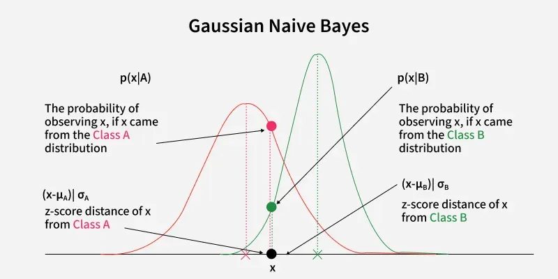
The formula for the Gaussian PDF is:

So, for each class, we will multiply its prior probability by the likelihoods of each feature under that class's specific Gaussian distributions. The class that yields the highest final value is our prediction.

A Practical Hurdle: Numerical Underflow

When you multiply many small numbers together (probabilities are always between 0 and 1), the result can become vanishingly small, a problem known as numerical underflow. This can cause the value to be rounded to zero by the computer, leading to incorrect calculations and instability.

The standard solution is to work with logarithms. Since the logarithm is a monotonically increasing function, maximizing a value is the same as maximizing its logarithm. That is, $\arg {\max }_{k}P(C_k|\mathbf{x})=\arg {\max }_k\log (P(C_k|\mathbf{x}))$.

By applying the log, our product of probabilities turns into a sum of log-probabilities, which is far more numerically stable:

This is the equation we will actually implement. For each new data point, we will calculate this "log-posterior" score for every class and predict the class with the highest score.

The following video provides an excellent walkthrough of this entire mathematical derivation, from the core formula to the crucial use of logarithms for stability.

Implementing the Prediction Logic

Now we are ready to add the predict method to our NaiveBayes class. The implementation will follow the logic we just derived. For each new sample, we'll compute the log-posterior score for each class and then use np.argmax to select the winning class.

A clean way to structure this is to create a helper method that computes the core log-likelihood term $\sum \log (P(x_i|C_k))$ for all classes.

The article below provides a clear, step-by-step implementation of the prediction logic.

Let's integrate this logic into our existing class structure from the previous lesson. We'll add a predict method and a helper method, _pdf, to calculate the Gaussian probability.

import numpy as np

class NaiveBayes:
    def fit(self, X, y):
        n_samples, n_features = X.shape
        self._classes = np.unique(y)
        n_classes = len(self._classes)

        self._means = np.zeros((n_classes, n_features), dtype=np.float64)
        self._variances = np.zeros((n_classes, n_features), dtype=np.float64)
        self._priors = np.zeros(n_classes, dtype=np.float64)

        for idx, c in enumerate(self._classes):
            X_c = X[y == c]
            self._means[idx, :] = X_c.mean(axis=0)
            self._variances[idx, :] = X_c.var(axis=0)
            self._priors[idx] = X_c.shape[0] / float(n_samples)




    # New methods for prediction
    def predict(self, X):
        y_pred = [self._predict_sample(x) for x in X]
        return np.array(y_pred)

    def _predict_sample(self, x):
        posteriors = []




        # Calculate posterior probability for each class
        for idx, c in enumerate(self._classes):
            prior = np.log(self._priors[idx])
            



            # Calculate log-likelihood
            likelihood = np.sum(np.log(self._pdf(idx, x)))
            
            posterior = prior + likelihood
            posteriors.append(posterior)




        # Return class with highest posterior probability
        return self._classes[np.argmax(posteriors)]

    def _pdf(self, class_idx, x):
        mean = self._means[class_idx]
        var = self._variances[class_idx]
        



        # Add a small epsilon for numerical stability in case variance is zero
        epsilon = 1e-4 
        
        numerator = np.exp(-((x - mean) ** 2) / (2 * (var + epsilon)))
        denominator = np.sqrt(2 * np.pi * (var + epsilon))
        
        return numerator / denominator

Let's break down the new code:

1. _pdf(self, class_idx, x): This helper method implements the Gaussian PDF formula. For a given class index and a single sample x, it retrieves the corresponding means and variances and computes the probability density for each feature. Note the addition of a small epsilon to the variance to prevent division by zero if a feature has zero variance in the training data for a particular class.
2. _predict_sample(self, x): This method computes the prediction for a single sample x.
   • It iterates through each class.
   • For each class, it calculates the log-prior.
   • It calls _pdf to get the likelihoods for each feature, takes their log, and sums them up to get the total log-likelihood.
   • It adds the log-prior and log-likelihood to get the final log-posterior score for that class.
   • After computing the scores for all classes, it uses np.argmax to find the index of the class with the highest score and returns the corresponding class label.
3. predict(self, X): This is the main public method. It takes a matrix of samples X and uses a list comprehension to call _predict_sample for each one, returning an array of predictions.

This completes our classifier! The calculations we just implemented define the decision boundaries of our model. For any given point in the feature space, the model calculates these posterior probabilities and assigns the point to the class with the highest score.

Conclusion

In this lesson, you've successfully implemented the prediction mechanism for a Gaussian Naive Bayes classifier. By combining the parameters learned during training with Bayes' theorem, you have built a complete, functional model from the ground up.

Key Takeaways:

• Prediction is MAP Estimation: We predict the class $C_k$ that maximizes the posterior probability $P(C_k|\mathbf{x})$.
• The Posterior is Proportional to Prior $\times$ Likelihood: The prediction logic combines the stored priors with the likelihood calculated from the data.
• Likelihood is from the Gaussian PDF: For each feature, the likelihood $P(x_i|C_k)$ is computed using the Gaussian PDF with the stored class-specific mean and variance.
• Log-Probabilities Ensure Stability: To avoid numerical underflow from multiplying small probabilities, we work with the sum of log-probabilities instead.
• The predict method encapsulates this entire process, using np.argmax to select the class with the highest log-posterior score.

In the next lesson, we will put it all together. You will apply and evaluate your custom-built Naive Bayes classifier on a standard dataset, testing its performance and seeing how our from-scratch model compares to established libraries.