Building and Evaluating a Naive Bayes Classifier

The Standard Machine Learning Workflow

Before we dive into the code, let's outline the process. Applying and evaluating a classifier, whether it's one you built yourself or one from a library like scikit-learn, typically follows these steps:

1. Load the Data: Obtain a dataset with features and corresponding class labels.
2. Split the Data: Divide the dataset into a training set (for the model to learn from) and a testing set (for unbiased evaluation).
3. Train the Model: Instantiate your classifier and call the fit method on the training data.
4. Make Predictions: Use the trained model's predict method on the features of the testing set.
5. Evaluate Performance: Compare the model's predictions with the true labels from the testing set using various metrics.

We will follow these exact steps using the NaiveBayes class you've built.

Applying Your Classifier to a Dataset

For this exercise, we will use the well-known Breast Cancer Wisconsin dataset, which is conveniently available through the scikit-learn library. This dataset contains continuous features describing cell nuclei, making it a perfect fit for our Gaussian Naive Bayes model.

The following video from the NeuralNine channel, which we used in our previous lesson, demonstrates this exact workflow. It will serve as a great practical guide as we walk through the steps.

Let's assemble the full script. We'll start with the complete NaiveBayes class from our previous lessons, then add the application and evaluation code.

import numpy as np
from sklearn.model_selection import train_test_split
from sklearn.datasets import load_breast_cancer
from sklearn.metrics import accuracy_score

# The complete NaiveBayes class from our previous lessons
class NaiveBayes:
    def fit(self, X, y):
        n_samples, n_features = X.shape
        self._classes = np.unique(y)
        n_classes = len(self._classes)

        self._means = np.zeros((n_classes, n_features), dtype=np.float64)
        self._variances = np.zeros((n_classes, n_features), dtype=np.float64)
        self._priors = np.zeros(n_classes, dtype=np.float64)

        for idx, c in enumerate(self._classes):
            X_c = X[y == c]
            self._means[idx, :] = X_c.mean(axis=0)
            self._variances[idx, :] = X_c.var(axis=0)
            self._priors[idx] = X_c.shape[0] / float(n_samples)

    def predict(self, X):
        y_pred = [self._predict_sample(x) for x in X]
        return np.array(y_pred)

    def _predict_sample(self, x):
        posteriors = []

        for idx, c in enumerate(self._classes):
            prior = np.log(self._priors[idx])
            likelihood = np.sum(np.log(self._pdf(idx, x)))
            posterior = prior + likelihood
            posteriors.append(posterior)

        return self._classes[np.argmax(posteriors)]

    def _pdf(self, class_idx, x):
        mean = self._means[class_idx]
        var = self._variances[class_idx]
        epsilon = 1e-4 # To avoid division by zero
        numerator = np.exp(-((x - mean) ** 2) / (2 * (var + epsilon)))
        denominator = np.sqrt(2 * np.pi * (var + epsilon))
        return numerator / denominator

# 1. Load the data
X, y = load_breast_cancer(return_X_y=True)

# 2. Split the data
X_train, X_test, y_train, y_test = train_test_split(X, y, test_size=0.2, random_state=42)

# 3. Train the model
nb_classifier = NaiveBayes()
nb_classifier.fit(X_train, y_train)

# 4. Make predictions
y_pred = nb_classifier.predict(X_test)

# 5. Evaluate performance
accuracy = accuracy_score(y_test, y_pred)
print(f"Accuracy of our custom Naive Bayes classifier: {accuracy:.4f}")

Running this script will train your classifier on 80% of the data and test it on the remaining 20%. The output will be the accuracy, which measures the proportion of correctly classified samples. You should see a score well above 90%, demonstrating that your from-scratch implementation is highly effective!

A Deeper Dive into Evaluation

As a data scientist, you know that accuracy, while useful, doesn't always tell the whole story, especially if the classes are imbalanced. To get a more complete picture of your model's performance, we can look at other metrics like the confusion matrix, precision, recall, and F1-score.

The following article provides a clear guide on implementing these evaluation steps.

Let's briefly define these key concepts:

• Confusion Matrix: A table that summarizes performance by showing the counts of:
  • True Positives (TP): Correctly predicted positive instances.
  • True Negatives (TN): Correctly predicted negative instances.
  • False Positives (FP): Incorrectly predicted as positive (Type I error).
  • False Negatives (FN): Incorrectly predicted as negative (Type II error).
• Precision: Of all the instances the model predicted as positive, what fraction were actually positive? It measures the "purity" of positive predictions.
  $\text{Precision}=\frac{\text{TP}}{\text{TP}+\text{FP}}$
• Recall (Sensitivity): Of all the actual positive instances, what fraction did the model correctly identify? It measures the model's ability to "find" all positive samples.
  $\text{Recall}=\frac{\text{TP}}{\text{TP}+\text{FN}}$
• F1-Score: The harmonic mean of precision and recall, providing a single score that balances both. It's particularly useful when you need to find a balance between minimizing both False Positives and False Negatives.
  $F_1=2\cdot \frac{\text{Precision}\cdot \text{Recall}}{\text{Precision}+\text{Recall}}$

By adding these metrics to our script, we get a much richer understanding of our classifier's behavior.

Visualizing the Model's "Thinking"

Now that we have quantitative measures of performance, let's connect them back to the internal mechanics of our model. During the fit phase, our model learned the mean and variance for each feature, for each class. This is equivalent to fitting a Gaussian distribution to the data for each feature-class combination.

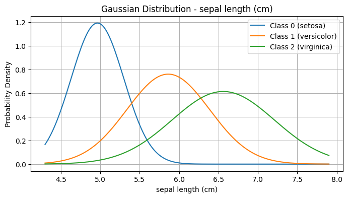
This plot shows the learned Gaussian distributions for a single feature across three different classes. When making a prediction, our model calculates the probability density from each of these curves for a new data point's feature value. The class with the highest combined probability (across all features) wins.

The predictions our model makes, and consequently the accuracy and confusion matrix, are the direct result of these learned distributions. The decision boundaries are the points in the feature space where the posterior probability is equal for two classes.

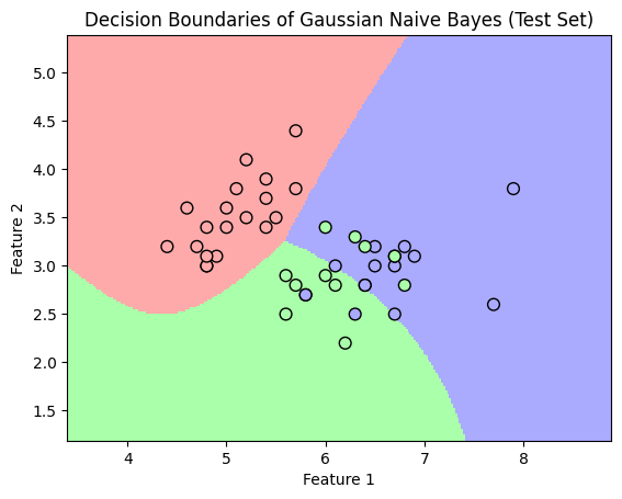
This plot illustrates the final decision boundaries learned by a Gaussian Naive Bayes classifier. Our evaluation metrics are quantifying how well these colored regions align with the true class labels of the test data points.

Conclusion

In this lesson, you have successfully brought your custom-built Gaussian Naive Bayes classifier to life. You applied it to a standard dataset, followed a real-world machine learning workflow, and evaluated its performance not just with accuracy, but with a comprehensive suite of metrics.

Key Takeaways:

• The standard ML workflow involves loading data, splitting it, training, predicting, and evaluating.
• Your from-scratch NaiveBayes class can be seamlessly integrated into this workflow.
• Accuracy is a good starting point for evaluation, but metrics like precision, recall, F1-score, and the confusion matrix provide deeper insights into a model's strengths and weaknesses.
• The model's performance is a direct consequence of the statistical parameters (priors, means, variances) it learns from the training data.

You have now completed the first module of this course, building a strong probabilistic foundation. In the next module, we will shift gears from supervised classification to unsupervised learning, beginning with a fundamental technique for Dimensionality Reduction and Data Visualization: Principal Component Analysis (PCA).