Frequentist vs. Bayesian Estimation

Welcome to the first lesson of your course on machine learning, NLP, and deep learning. We're starting with a module on probabilistic foundations, which will provide the mathematical and conceptual groundwork for many of the advanced models we'll explore later.

This lesson tackles a fundamental, and somewhat philosophical, division in the world of statistics and machine learning. Your goal is to be able to explain the difference between the frequentist and Bayesian approaches to parameter estimation. Understanding this distinction is crucial because it underlies the design of many algorithms, from simple linear regression to complex neural networks. We'll see how different loss functions and regularization techniques, which you're already familiar with from your data science experience, can often be interpreted through one of these two lenses.

Two Views on Probability

At its heart, the debate between frequentists and Bayesians stems from two different interpretations of what probability means.

Frequentist View: Probability is the long-run frequency of a repeatable event. If you flip a coin infinitely many times, the probability of heads is the fraction of times it came up heads. In this view, model parameters (like the true bias of a coin) are considered fixed, unknown constants. Our goal is to use data to calculate a single best estimate of these constants.
Bayesian View: Probability is a degree of belief about a statement, which can be updated as we gather more evidence. Parameters are treated as random variables themselves, which have their own probability distributions. We start with a prior belief about a parameter and use data to update it into a posterior belief.

This image provides a concise summary of these contrasting philosophies.

A high-level comparison of the Frequentist and Bayesian schools of thought. The frequentist view defines probability as long-run frequency and sees parameters as fixed, while the Bayesian view defines probability as a degree of belief and treats parameters as having their own distributions.

Let's now see how these philosophies translate into two different methods for estimating parameters from data.

The Frequentist Approach: Maximum Likelihood Estimation (MLE)

The quintessential frequentist method for parameter estimation is Maximum Likelihood Estimation (MLE). The name says it all: we want to find the parameter value(s) that make our observed data most likely.

Imagine you're trying to model a noisy signal, a scenario that should be familiar from your ECE background. You have a model, but you need to determine its parameters (e.g., the amplitude of the underlying signal). MLE asks: "Which parameter value would maximize the probability of observing the exact noisy data that we collected?"

The function we maximize is called the likelihood function, denoted $P (data ∣ θ)$ , where $θ$ represents the parameter(s) we want to estimate. The MLE estimate is the value of $θ$ that maximizes this function:

θ_{MLE} = θ ar g max P (data ∣ θ)

To see this in action, the following video provides an excellent visual and mathematical walkthrough. It uses an example of estimating a parameter x from a noisy measurement y where the noise is Gaussian—a classic signal processing problem.

What are Maximum Likelihood (ML) and Maximum a posteriori (MAP)? ("Best explanation on YouTube")

Watch the first part of this video from "Iain Explains Signals, Systems, and Digital Comms" to understand the mechanics of MLE.

Focus on the segment from the definition of MLE to the derivation for the Gaussian example. Pay close attention to the visual explanation of how MLE finds the parameter (x) corresponding to the Gaussian distribution that has its peak at the observed data point (y_bar).

As the video demonstrates, for many common problems, the MLE result is very intuitive. For a series of coin flips, the MLE for the probability of heads is simply the number of heads divided by the total number of flips. For a Gaussian distribution, the MLE for the mean is the sample mean of the data.

However, MLE has a potential weakness: it relies only on the observed data. If you flip a coin three times and get heads each time, MLE concludes the coin's probability of heads is 1.0. While this is the most likely parameter given only that data, our intuition tells us this is an overreaction to a small sample size. This is where the Bayesian approach comes in.

The Bayesian Approach: Incorporating Prior Beliefs

Bayesians address the limitations of MLE by incorporating prior knowledge. They argue that we rarely start with a completely blank slate. We might believe that most coins are fair, or that a physical parameter must be positive. This is formalized using Bayes' Theorem.

To see how Bayes' theorem is adapted from a simple rule of probability to a powerful tool for statistical inference, watch the following short video.

The better way to do statistics | Bayesian #1

This video from the channel "Very Normal" will introduce how Bayes' Theorem forms the foundation of Bayesian statistics.

Watch the section from statistical inference. The key is to understand how the theorem is re-framed with data and parameters, and to grasp the meaning of the three core components: the prior, the likelihood, and the posterior.

As the video explained, the Bayesian approach updates our beliefs. In the context of parameter estimation, Bayes' Theorem is written as:

P (θ ∣ data) = \frac{P ( data ∣ θ ) P ( θ )}{P ( data )}

Or, since the denominator $P (data)$ is a normalizing constant that doesn't depend on $θ$ , we can simplify this to a proportionality:

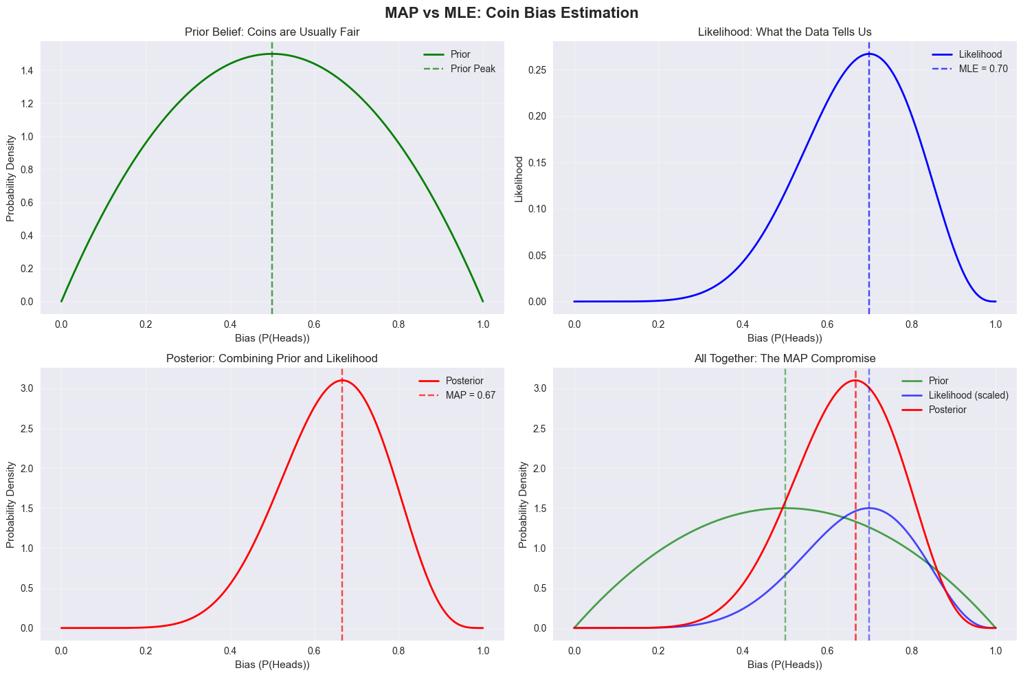
Posterior P (θ ∣ data) \propto Likelihood P (data ∣ θ) \times Prior P (θ)

Prior $P (θ)$ : Our belief about the parameter $θ$ before seeing any data. For a coin, we might use a prior that puts most of its weight around $θ = 0.5$ .
Likelihood $P (data ∣ θ)$ : The same function used in MLE. It represents how likely the data is, given a specific parameter value.
Posterior $P (θ ∣ data)$ : Our updated belief about $θ$ after considering the data. It represents a compromise between our prior belief and the evidence from the data.

This leads to two forms of Bayesian estimation.

1. Maximum A Posteriori (MAP) Estimation

The most direct parallel to MLE is Maximum A Posteriori (MAP) estimation. Instead of maximizing just the likelihood, MAP finds the parameter value that maximizes the entire posterior probability.

θ_{MAP} = θ ar g max P (θ ∣ data) = θ ar g max [P (data ∣ θ) P (θ)]

Notice that if we choose a "flat" or uniform prior (i.e., we assume all parameter values are equally likely, $P (θ) = constant$ ), then maximizing the posterior is the same as maximizing the likelihood, and $θ_{MAP} = θ_{MLE}$ . In this sense, MLE is a special case of MAP.

The connection to your existing knowledge of machine learning is very strong here. Adding a regularization term to a model's loss function is often mathematically equivalent to performing MAP estimation. For example, minimizing a mean squared error loss with L2 regularization is equivalent to finding the MAP estimate of the model weights, assuming a Gaussian prior on those weights. The prior "pulls" the weights towards zero, preventing them from overfitting to the data, just as a prior belief about a fair coin would pull the estimate away from 1.0 even if we see three heads in a row.

Now, let's return to the video you watched earlier to see how it extends the MLE concept to MAP.

What are Maximum Likelihood (ML) and Maximum a posteriori (MAP)? ("Best explanation on YouTube")

Watch the second part of the "Iain Explains" video to see how MAP builds upon MLE.

Watch from the introduction of prior knowledge. The key takeaway is how the prior distribution, f(x), is used to "weight" the likelihood, resulting in an estimate that balances prior knowledge with observed data.

2. Full Bayesian Inference

While MAP gives us a single point estimate (just like MLE), it doesn't capture the full richness of the Bayesian approach. The ultimate goal of Bayesian inference is not just to find the single most probable parameter, but to determine the entire posterior distribution, $P (θ ∣ data)$ .

This distribution is the complete output. From it, we can calculate a point estimate if we wish (e.g., the mode of the distribution is the MAP estimate), but we also get a measure of our uncertainty. A narrow posterior distribution means we are very confident in our estimate, while a wide distribution signifies high uncertainty.

Let's explore this using a clear example involving a coin toss.

Full Explanation of MLE, MAP and Bayesian Inference

This article from Towards Data Science provides a great walkthrough of all three concepts using a consistent coin-toss example.

First, read the introduction to familiarize yourself with the notation: Introducing the concepts. Then, skim the section on MAP to see how a Beta distribution is introduced as a prior: MAP with a prior. Finally, and most importantly, read the sections that compare the methods and explain the unique benefit of full Bayesian inference: start at Discussion of Results and continue through the "game show" example to Why Bayesian Inference is powerful.

The "game show" example in the article is the perfect illustration of why a full posterior distribution is more informative than a single point estimate. Both coins have a MAP estimate of 0.5, but the posterior distributions reveal that we are far more certain about the fairness of the coin that was flipped 1000 times.

The following image visualizes the entire process for the coin bias example, showing how the prior belief is combined with the likelihood from the data to form the posterior belief. The peaks of the likelihood and posterior correspond to the MLE and MAP estimates, respectively.

This figure illustrates the components of Bayesian estimation. The Prior (green) reflects our initial belief that coins are usually fair. The Likelihood (blue) is derived from the data (e.g., observing 70 heads in 100 flips), with its peak at the MLE of 0.7. The Posterior (red) is the result of combining the prior and likelihood; its peak is the MAP estimate of 0.67, a compromise between the prior's peak (0.5) and the MLE.

Summary of Differences

Let's consolidate the key distinctions:

Feature	Frequentist (e.g., MLE)	Bayesian (e.g., MAP, Full Inference)
View of Parameters	Fixed, unknown constants.	Random variables with distributions.
View of Probability	Long-run frequency of events.	Degree of belief.
Core Idea	Find parameters that maximize the likelihood of the data.	Use data to update prior beliefs into posterior beliefs.
Inputs	Data only.	Data and a prior distribution.
Output	A single point estimate.	A point estimate (MAP) or a full posterior distribution.
Quantifying Uncertainty	Indirectly, via confidence intervals.	Directly, via the variance of the posterior distribution.

Conclusion

In this lesson, you've explored the two dominant philosophies of parameter estimation. The frequentist approach, exemplified by MLE, seeks the single set of fixed parameters that best explains the data. The Bayesian approach, using MAP or full inference, treats parameters as variables themselves and updates our beliefs about them, providing not just an estimate but a measure of uncertainty.

As we move forward, you will see these ideas in action. Many standard machine learning models are implicitly frequentist, where training involves finding the MLE of the parameters. Techniques like regularization can be viewed as a bridge to the Bayesian world, introducing priors to guide the learning process.

In the next lesson, we will get our hands dirty with the mathematics of MLE. You will derive the Maximum Likelihood Estimation for the parameters of a Gaussian distribution, a foundational skill for understanding many probabilistic models.

Recommended resources