Welcome back! In our previous lesson, we established the fundamental organizational structure of electrons within an atom, moving from the broad concept of shells to the more specific subshells and orbitals. We now know how many orbitals exist within the s, p, and d subshells. Today, we'll bring that abstract framework to life.
This lesson focuses on the second part of your initial goal: building a strong visual and conceptual foundation. We will visualize and describe the distinct three-dimensional shapes of the s, p, and d orbitals and understand how they are oriented in space. This will complete our exploration of the atom's "architecture" before we learn the rules for filling it with electrons.
From Numbers to Shapes: An Intuitive Origin
Before we just memorize the shapes, it's helpful to understand where they come from. You have a background in physics, so you'll appreciate that these shapes aren't arbitrary; they are the result of the wave-like nature of electrons. An orbital is best thought of as a 3D probability map—a region where an electron is most likely to be found. These probability maps are essentially three-dimensional standing waves.
A fantastic video from the channel FloatHeadPhysics provides an intuitive explanation for why these standing waves produce the specific shapes we observe. It uses an analogy of waves on a string to build up the shapes of s, p, and d orbitals.
I finally understood orbital shapes intuitively! (My mind is blown)
This video connects the physics of standing waves to the chemistry of atomic orbitals, providing a deep, intuitive understanding of their shapes.
Watch the following segments in order: First, watch the introduction to the core idea, which frames electrons as probability waves. Next, see how the simple analogy of a confined wave on a string leads to discrete energy levels and the concept of nodes (points of zero amplitude). This is key: more nodes mean higher energy. See this applied to the simplest 3D case, the hydrogen atom's ground state, which results in a spherical probability map. This is the fundamental s orbital. You can skip the analogy about tracking a child from 00:10:06 to 00:12:09 if you wish, as it reinforces the same point. The next level of energy introduces a node. The video explains how introducing a flat, or planar, node by slicing the sphere creates the characteristic dumbbell shape of a p orbital. Notice how three possible slices lead to three possible p orbitals. Following this logic, see how introducing two angular nodes (two planar slices) results in the four-lobed shape of a d orbital. Finally, watch the summary that ties the orbital's shape directly to the number of angular nodes.
From this video, we can extract a powerful idea: the complexity and shape of an orbital are determined by the number of specific nodes it has.
- 0 angular nodes: Results in a spherical shape (s orbital).
- 1 angular node: Results in a dumbbell shape (p orbital).
- 2 angular nodes: Results in a cloverleaf-like shape (d orbital).
Now that we have the intuition, let's examine the specific shapes and their orientations in detail.
The Atlas of Atomic Orbitals: s, p, and d
Chemists use a standard set of representations for these orbitals, oriented within a 3D Cartesian coordinate system (x, y, z). The image below provides a complete overview of the shapes we will discuss.
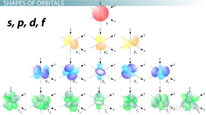
The s Orbital: Spherical and Simple
As we saw, the simplest orbital is the s orbital.
- Shape: It is spherically symmetrical. This means the probability of finding the electron depends only on its distance from the nucleus, not on the direction.
- Orientation: Being a perfect sphere, it has no directional preference. There is only one
sorbital per energy level. - Size: The size of the
sorbital increases as the principal quantum number (n) increases. So, a2sorbital is larger than a1sorbital, and a3sis larger than a2s.
The following reading provides excellent visuals and descriptions for the s, p, and d orbitals.
6.6: The Shapes of Atomic Orbitals - Chemistry LibreTexts
This resource from Chem LibreTexts contains clear diagrams and concise descriptions of the orbital shapes and their key features, like nodes.
Start by reading the section on s Orbitals. Note Figure 6.6.2, which shows how the 1s, 2s, and 3s orbitals increase in size and also develop internal spherical nodes (which we saw in the video). Then, move to the section on p Orbitals and study Figures 6.6.3 and 6.6.4, which illustrate the dumbbell shape and the nodal plane at the nucleus. Finally, read the section on d Orbitals and examine Figure 6.6.5, which shows the five distinct d orbital shapes.
The p Orbitals: Dumbbells in Space
Beginning with the second energy level (n=2), we encounter the p subshell, which contains three p orbitals.
- Shape: Each
porbital has a dumbbell shape, consisting of two lobes on opposite sides of the nucleus. - Node: There is a nodal plane at the nucleus, where the probability of finding the electron is zero. This plane separates the two lobes.
- Orientation: The three
porbitals are oriented perpendicularly to each other, aligned along the x, y, and z axes. They are designatedp_x,p_y, andp_zbased on the axis they lie on. These three orbitals are degenerate, meaning they have the same energy.
The d Orbitals: Complex and Critical
Starting at the third energy level (n=3), we find the d subshell, which contains five d orbitals. These are crucial for understanding the chemistry of transition metals. Their shapes are more complex, but their names are quite descriptive.
To get a formal description of their names and orientations, let's consult a text from Purdue University's chemistry department.
Quantum Numbers and Electron Configurations
This resource provides a concise, text-based description of the five d orbitals, giving their official names and describing their positions relative to the Cartesian axes.
Please read the paragraph that begins with this sentence. This will explicitly name and describe the orientation of the five 3d orbitals.
The five d orbitals are:
d_xy,d_yz, andd_xz: These three orbitals look like four-leaf clovers, with their lobes located between the axes indicated in their name (e.g., thed_xyorbital lobes lie in the xy-plane, between the x and y axes).d_(x^2-y^2): This orbital also has a clover shape, but its lobes are oriented directly along the x and y axes.d_(z^2): This orbital has a unique shape: a dumbbell shape along the z-axis with a "donut" or torus of electron density in the xy-plane.
Though they look different, all five d orbitals in a given subshell are degenerate. Visualizing these can be challenging from static images. The following 3D animation is extremely helpful.
Shape and Size of Orbitals 3D Visualisation
This short video from the channel aahnik provides clear, rotating 3D models of the p and d orbitals, making their spatial orientations easy to understand.
First, watch the visualization of the three p orbitals from px, py, and pz. Then, watch the detailed visualizations of each of the five d orbitals, presented one by one from dxy to dz^2.
Conclusion
Today we have moved from the numerical rules of electron organization to a visual, three-dimensional understanding of where electrons are likely to be found. You can now connect the abstract labels s, p, and d to concrete shapes and spatial arrangements.
Here are the key takeaways:
- Orbital Shapes: Orbitals are probability maps with distinct shapes determined by their subshell type.
sorbitals are spherical,porbitals are dumbbell-shaped, anddorbitals have more complex, mostly four-lobed shapes. - Spatial Orientation:
sorbitals are non-directional. The threeporbitals (p_x,p_y,p_z) are oriented along the Cartesian axes. The fivedorbitals have specific orientations either along or between the axes. - Nodes: The shapes are a consequence of nodes in the electron's wave function.
sorbitals have 0 angular nodes,phave 1, anddhave 2.
We have now established the "what" and "where" of atomic orbitals. In our next lesson, we will address the "how." We'll learn the three fundamental rules—the Aufbau principle, the Pauli exclusion principle, and Hund's rule—that govern how electrons fill these orbitals. This will allow us to start building electron configurations for actual elements.