Taming the Event Horizon: Kruskal-Szekeres Coordinates

1. A Coordinate Problem or a Physical Catastrophe?

Our first task is to determine whether the breakdown at $r=2M$ signifies a genuine physical singularity, where spacetime itself is destroyed, or merely a pathology of our chosen coordinate system, much like the singularity at the origin of polar coordinates.

A powerful tool for this diagnosis is a curvature invariant. Since a scalar quantity's value is independent of the coordinate system used to compute it, if a scalar constructed from the Riemann curvature tensor diverges, we know we've found a true physical singularity. If all such scalars remain finite, the problem is likely with our coordinates.

The simplest invariant, the Ricci scalar $R$, is zero everywhere for a vacuum solution like Schwarzschild's, so it's not helpful. The next simplest is the Kretschmann scalar, $K=R_{\mu \nu \rho \sigma }{R}^{\mu \nu \rho \sigma }$.

As the notes show, the Kretschmann scalar for the Schwarzschild metric is:

Let's analyze its behavior at our two points of concern:

• At the center ($r\to 0$): $K\to \infty$. The curvature blows up. This is a genuine physical singularity. Our theory of gravity breaks down here.
• At the horizon ($r\to 2M$): $K=\frac{48M^2}{(2M{)}^6}=\frac{3}{4M^4}$. This value is perfectly finite.

This is our smoking gun: the "singularity" at the event horizon is an illusion created by a poor choice of coordinates. The spacetime geometry itself is well-behaved there. Our task is now to find a better coordinate system that doesn't break down.

2. A Stepping Stone: Eddington-Finkelstein Coordinates

Before constructing the complete solution, let's explore a simpler coordinate system that already "heals" the horizon for observers or light rays falling into the black hole. The strategy is to define a new time coordinate based on the path of an ingoing light ray.

This requires introducing the tortoise coordinate, $r_{\ast }$, defined by the differential relation:

Integrating this gives:

Notice that as the radial coordinate $r$ approaches the horizon $2M$, the tortoise coordinate $r_{\ast }$ goes to $-\infty$. The event horizon is infinitely far away in this new radial measure, which explains why in Schwarzschild coordinates, we see an infalling object take an infinite amount of time to reach it.

We now define new null coordinates based on $r_{\ast }$. These coordinates are designed to follow the paths of light rays.

Let's summarize the key results from the video.

By defining an "advanced time" coordinate $v=t+r_{\ast }$, which is constant along ingoing radial null geodesics, we can transform the Schwarzschild metric into the ingoing Eddington-Finkelstein form:

This metric is now perfectly regular at $r=2M$. The determinant is $-r^4{\sin }^2\theta$, which is non-zero away from the singularity at $r=0$. This coordinate system successfully extends the spacetime manifold to include the region $r\le 2M$.

The most profound consequence is seen in the behavior of the light cones. As the video illustrates, as an object approaches and crosses $r=2M$, its future light cone "tips over" such that it points entirely toward smaller values of $r$. Once inside, all possible future paths, even for light, lead inevitably to the central singularity at $r=0$. The event horizon is a true one-way membrane.

As the video and Tong's notes also discuss, we could have instead defined outgoing Eddington-Finkelstein coordinates using $u=t-r_{\ast }$. This would give us a coordinate patch describing a white hole—a time-reversed black hole from which matter is expelled.

The fact that we have two different, incompatible extensions (a black hole and a white hole) tells us we still haven't captured the full picture. We need a coordinate system that covers both.

3. The Maximal Extension: Kruskal-Szekeres Coordinates

Our goal is to find a set of coordinates where the metric is regular everywhere except the true singularity at $r=0$. The strategy, developed by Martin Kruskal and George Szekeres, is to perform a clever exponential transformation on the null coordinates $u$ and $v$. This is designed to precisely cancel out the problematic factor of $(1-2M/r)$ in the metric.

The derivation is mathematically involved, but the logic is beautiful.

Let's lay out the resulting coordinate transformation. For the region outside the horizon ($r>2M$), the Kruskal-Szekeres coordinates $(T,X)$ are related to the Schwarzschild coordinates $(t,r)$ by:

Inside the horizon ($r<2M$), the roles of the hyperbolic functions switch:

In these new coordinates, the Schwarzschild line element takes the strikingly simple form:

Here, $r$ is implicitly defined as a function of $T$ and $X$ by the relation $X^2-T^2=(\frac{r}{2M}-1)e^{r/2M}$.

The crucial feature is that the $(-d{T}^2+d{X}^2)$ part is just the 2D Minkowski metric. The entire metric is the Minkowski metric multiplied by a conformal factor that is positive and finite everywhere except at $r=0$. We have successfully found coordinates that cover the entire spacetime manifold and are regular everywhere except at the true physical singularity. This is called the maximal analytic extension of the Schwarzschild spacetime.

4. The Kruskal Diagram and Its Revelations

The $(T,X)$ plane is known as the Kruskal-Szekeres diagram. It reveals the complete causal structure of the spacetime.

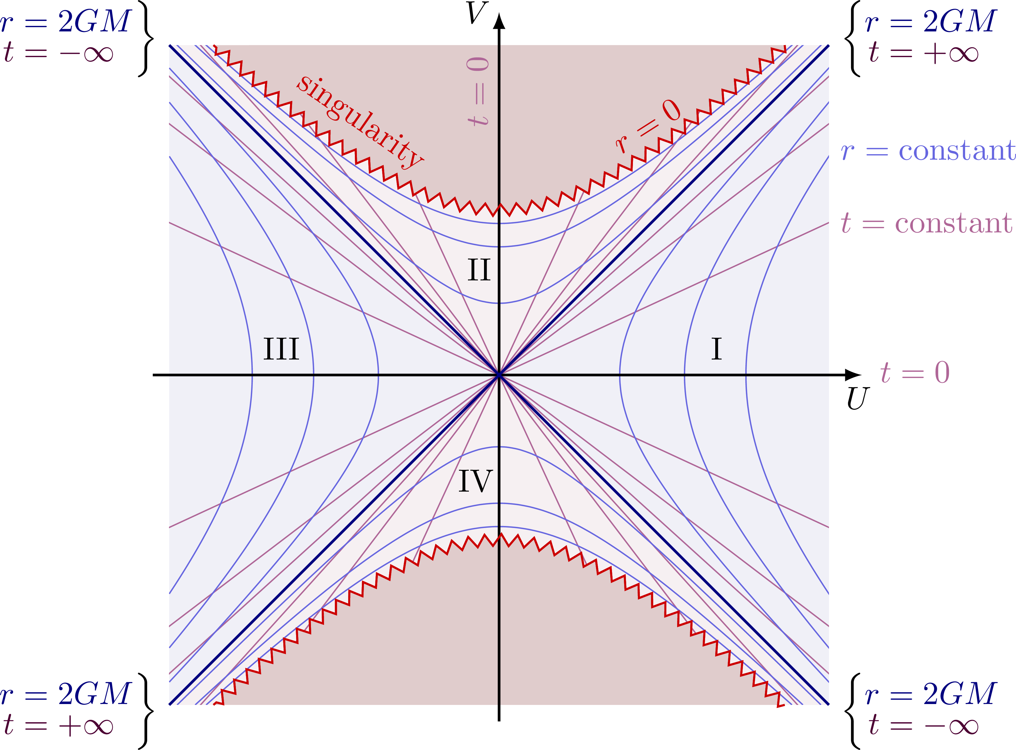
Let's analyze this remarkable map.

Here's a breakdown of the key features revealed on the diagram:

• Light Rays: Since the $(T,X)$ part of the metric is conformally flat, radial null geodesics are straight lines at 45 degrees ($T=\pm X+\text{const}$).
• The Singularity ($r=0$): This corresponds to the hyperbolas $T^2-X^2=1$. Notice there are two: a future singularity at the top ($T>0$) and a past singularity at the bottom ($T<0$).
• The Event Horizon ($r=2M$): This corresponds to $T^2-X^2=0$, or the diagonal lines $T=\pm X$.
• The Four Regions:
  • Region I (Right Quadrant, $X>|T|$): This is our universe, the asymptotically flat region covered by the original Schwarzschild coordinates.
  • Region II (Top Quadrant, $T>|X|$): This is the black hole interior. Any worldline entering this region (by crossing the future event horizon $T=X$) must end on the future singularity ($T^2-X^2=1,T>0$). Notice that inside this region, surfaces of constant $r$ are spacelike, while surfaces of constant $t$ are timelike. The roles have swapped! The singularity at $r=0$ is not a place in space; it is a moment in the future that is unavoidable.
  • Region IV (Bottom Quadrant, $T<-|X|$): This is the white hole interior. It is the time-reversal of the black hole. All worldlines in this region must have originated from the past singularity.
  • Region III (Left Quadrant, $X<-|T|$): This is another, completely separate asymptotically flat region. It represents a "parallel universe".

Regions I and III are connected by a non-traversable wormhole known as the Einstein-Rosen bridge. An observer starting in Region I cannot reach Region III because they would have to travel faster than light.

It is important to note that the white hole and the parallel universe are features of the eternal black hole solution. For a physical black hole formed from the collapse of a star, these regions are not believed to exist; the collapsing matter effectively cuts them out of the spacetime diagram. Nevertheless, the Kruskal solution is invaluable for understanding the complete mathematical structure of the geometry.

Conclusion

We have taken a deep dive into the causal structure of the Schwarzschild spacetime, moving far beyond what our original coordinates could show us.

Key Takeaways:

• The singularity at the event horizon $r=2M$ is a coordinate singularity, confirmed by the finiteness of the Kretschmann scalar. The singularity at $r=0$ is a true physical singularity.
• Eddington-Finkelstein coordinates provide a partial fix by extending the manifold across the horizon, revealing its "one-way membrane" nature where light cones tip inwards.
• Kruskal-Szekeres coordinates provide the maximal analytic extension of the spacetime, removing the coordinate singularity and revealing a structure with four distinct regions.
• The Kruskal diagram shows a black hole interior (Region II), a white hole interior (Region IV), and two asymptotically flat exterior regions (I and III) connected by a non-traversable wormhole.
• Inside the black hole's event horizon, the radial coordinate $r$ becomes timelike and the time coordinate $t$ becomes spacelike. The singularity at $r=0$ is an inevitable future moment, not a location in space.

Preview of Next Lesson:

The Kruskal diagram is a complete map, but its coordinate axes stretch to infinity. To better visualize the global causal structure and the nature of infinity itself, we can perform one final transformation that "squashes" the entire infinite diagram into a finite shape. In our next lesson, we will construct the Penrose diagram for the maximally extended Schwarzschild spacetime, a powerful tool for understanding causality at a glance.