Primordial Power Spectrum Calculation

Hello! Welcome to your next lesson in our exploration of Cosmological Perturbation Theory.

In our last lesson, we established the profound idea that the vast structures of our universe originate from quantum fluctuations of the inflaton field. We used a powerful physical argument—the "time-delay" mechanism—to derive the leading-order, scale-invariant power spectrum of curvature perturbations: $P_{ζ} \approx \frac{1}{2 ϵ M _{P l}^{2}} (\frac{H}{2 π})^{2}$ . This result captures the essence of the mechanism but relies on the approximation that inflation is a perfect de Sitter expansion, where $H$ and $ϵ$ are constant.

Today, we will go beyond this approximation to achieve the lesson's learning outcome: to calculate the power spectrum of primordial curvature perturbations generated during inflation, including the all-important deviations from perfect scale-invariance. This requires a fully rigorous calculation, which will satisfy your preference for deep mathematical formalism while yielding one of the most precise and successful predictions in all of physics.

1. Defining the Power Spectrum and Spectral Tilt

The power spectrum, $P_{ζ} (k)$ , quantifies the "power" or variance of the curvature fluctuations on a given comoving scale, represented by the wavenumber $k$ . It is formally defined from the two-point correlation function of the curvature perturbation in Fourier space:

⟨ ζ_{k} ζ_{k^{'}} ⟩ = (2 π)^{3} δ^{(3)} (k + k^{'}) \frac{2 π ^{2}}{k ^{3}} P_{ζ} (k)

The prefactor $\frac{2 π ^{2}}{k ^{3}}$ is chosen so that a perfectly scale-invariant spectrum, where the variance per logarithmic interval in $k$ is constant, corresponds to $P_{ζ} (k) = const$ .

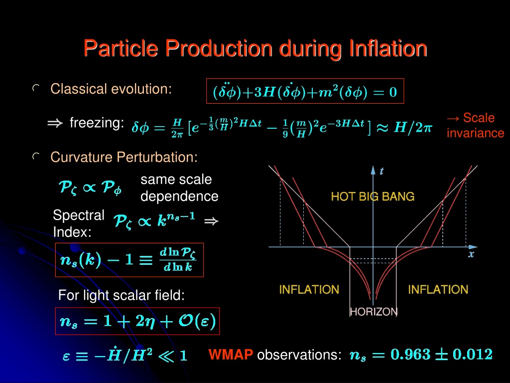
However, since inflation is not eternal and the inflaton field rolls down its potential, we expect small deviations from perfect scale invariance. These are parameterized by the scalar spectral index, $n_{s}$ , defined via a power-law approximation:

P_{ζ} (k) = A_{s} (\frac{k}{k _{0}})^{n_{s} - 1}

Here, $A_{s}$ is the amplitude of the spectrum at some pivot scale $k_{0}$ .

$n_{s} = 1$ : A perfectly scale-invariant (Harrison-Zel'dovich) spectrum. Fluctuations have the same amplitude on all scales.
$n_{s} < 1$ : A "red-tilted" spectrum. There is more power on large scales (small $k$ ) than on small scales (large $k$ ).
$n_{s} > 1$ : A "blue-tilted" spectrum. There is more power on small scales.

Observations from the Cosmic Microwave Background (CMB) have measured these parameters with incredible precision.

Power Spectrum of Primordial Curvature Perturbations — This image shows the definition of the primordial power spectrum $P_\zeta(k)$, its power-law parameterization, and the values for the amplitude and spectral index as measured by the WMAP7 satellite. The slight deviation of $n_s$ from 1 is a crucial piece of evidence supporting inflation.

2. An Intuitive Derivation of the Spectral Tilt

Before diving into the full field-theoretic calculation, let's build our intuition. The physical reason for the tilt is that the background quantities $H$ and $ϕ ˙$ are not truly constant; they evolve slowly as the inflaton rolls. Different Fourier modes $k$ exit the Hubble horizon at slightly different times, and thus they "freeze out" with an amplitude determined by the values of $H$ and $ϕ ˙$ at that specific moment.

This time dependence translates directly into the scale dependence of the power spectrum. The following reading from Leonardo Senatore's lecture notes walks through this elegant argument.

Lectures on Inflation Introduction

These notes provide a concise, heuristic derivation of the spectral tilt by considering the slow evolution of the Hubble parameter and the inflaton's velocity during inflation.

Please read Section 2.4, 'Scale invariance and tilt' (pages 23-24). The key is to understand how evaluating the power spectrum at the moment of horizon crossing, k = aH, introduces a k-dependence. Follow the chain rule argument in Eq. (90) that leads to the result for n_s - 1.

The core of the argument is to take our leading-order formula for the power spectrum, $P_{ζ} (k) \propto H^{4} / ϕ ˙^{2}$ , and recognize that the right-hand side should be evaluated at the time of horizon-crossing, $t_{k}$ , for each mode $k$ . The spectral index is then given by the logarithmic derivative:

n_{s} - 1 = \frac{d ln P _{ζ}}{d ln k}_{k = a H} = \frac{d ln ( H ^{4} / ϕ ˙ ^{2} )}{d t} \frac{d t}{d ln k}_{k = a H}

Using $d ln k \approx d ln (a H) \approx H d t$ , we can relate the derivative with respect to $k$ to a time derivative. Expressing the time derivatives of $H$ and $ϕ ˙$ in terms of the slow-roll parameters $ϵ = - \frac{H ˙}{H ^{2}}$ and $η = M_{P l}^{2} \frac{V ^{''}}{V}$ eventually yields the standard result:

n_{s} - 1 = 2 η - 6 ϵ

This crucial formula connects a directly observable cosmological parameter, $n_{s}$ , to the fundamental parameters describing the shape of the inflaton potential.

3. The Rigorous Calculation

We now have the physical intuition and the expected answer. It is time to perform the full, rigorous calculation. This involves quantizing the coupled system of scalar field fluctuations and metric perturbations. As you know from your study of gauge theories, dealing with gauge redundancy is a subtle business. The standard approach is to fix a gauge, identify the true physical degree of freedom, and quantize its dynamics.

The lecture notes by Senatore provide an exceptionally clear and modern derivation using the "Effective Field Theory of Inflation" formalism. We will work in the so-called $π$ -gauge, or unitary gauge.

Lectures on Inflation Introduction

This is the heart of today's lesson. This section provides a complete, step-by-step derivation of the power spectrum from first principles, correctly handling the subtleties of quantizing fluctuations in an expanding spacetime.

Please study Section 3.6, 'Rigorous calculation of the power spectrum in π-gauge' (pages 49-52). This is a dense but rewarding section. Focus on the following key steps: The Setup: Understand the ADM parametrization of the metric and how the inflaton fluctuation is represented by the field \pi(x,t) in the action (Eq. 189). Constraint Equations: Note that the equations of motion for the lapse N and shift N^i have no time derivatives. This is crucial: they are not independent degrees of freedom but are constrained by the dynamics of \pi. Gauge Fixing: See how fixing the gauge to h_{ij} = a^2 \delta_{ij} allows one to solve the constraint equations for N and N^i in terms of \pi (Eq. 194). The Master Action: Realize that substituting these solutions back into the original action yields a simple quadratic action for a single scalar field, \pi (Eq. 195). This is the main achievement of the procedure. Quantization: Follow the standard canonical quantization procedure for the \pi field: find the conjugate momentum, impose commutation relations, and expand in creation/annihilation operators. Solving for the Mode Function: The equation of motion for the classical mode function \pi_k^{cl} is solved with the Bunch-Davies vacuum condition, which specifies the state in the short-wavelength (flat-space) limit. Final Result: Track how the solution for \pi_k^{cl} is used to find the curvature perturbation \zeta_k = -H \pi_k, and how its two-point function leads directly to the final power spectrum (Eq. 206).

The final result of this rigorous calculation is:

⟨ ζ_{k} ζ_{k^{'}} ⟩_{late} = (2 π)^{3} δ^{(3)} (k + k^{'}) \frac{1}{k ^{3}} \cdot \frac{H _{f . o .}^{4}}{4 ( - H ˙ _{f . o .} ) M _{P l}^{2}}

where the subscript "f.o." means the quantities are evaluated at freeze-out (horizon crossing, $k = a H$ ).

From this, we can read off the power spectrum:

P_{ζ} (k) = \frac{H _{k}^{4}}{4 ( - H ˙ _{k} ) M _{P l}^{2}} = \frac{H _{k}^{2}}{4 ϵ _{k} M _{P l}^{2}}

Comparing this to our heuristic result from the previous lesson, $P_{ζ} = \frac{1}{2 ϵ M _{P l}^{2}} (\frac{H}{2 π})^{2}$ , we see they match perfectly after accounting for the factor of $(2 π)^{2}$ . The rigorous derivation gives:

P_{ζ} (k) = \frac{1}{2 ϵ _{k} M _{P l}^{2}} (\frac{H _{k}}{2 π})^{2}

This confirms our previous result, but now it stands on the solid ground of a full quantum field theory calculation in curved spacetime. The $k$ subscripts emphasize that all quantities are evaluated when the mode $k$ crosses the horizon.

Test your understanding!

In the derivation from Senatore's notes, the action for the $π$ field (Eq. 195) contains a mass-like term $- 3 H ˙ π^{2}$ . However, in the subsequent steps to solve for the mode function, this term is neglected. Why is this a valid approximation at leading order? (Hint: Think about the relative size of this term compared to the kinetic terms during inflation).

Show answer

The full equation of motion for $π_{k}$ from the action in Eq. (195) would be (after Fourier transform and some manipulation):

π ¨_{k} + 3 H π ˙_{k} + \frac{k ^{2}}{a ^{2}} π_{k} + (3 H ˙ + other terms) π_{k} = 0

The "mass" term is proportional to $H ˙$ , which can be written as $- ϵ H^{2}$ . The term is of order $ϵ H^{2}$ .
Let's compare this to the main dynamical term, $k^{2} / a^{2}$ . At horizon crossing, $k / a \sim H$ . Well inside the horizon ( $k / a ≫ H$ ), the $k^{2} / a^{2}$ term dominates, and the mass term is negligible. The mode oscillates freely.
Well outside the horizon ( $k / a ≪ H$ ), both the $k^{2} / a^{2}$ and mass terms are small compared to the Hubble friction term $3 H π ˙_{k}$ . In this regime, the solution freezes out.
The mass term's primary effect is to slightly modify the evolution around the time of horizon crossing. Since $ϵ$ is a small slow-roll parameter ( $ϵ ≪ 1$ ), the mass term $\sim ϵ H^{2}$ is a small correction compared to the energy scale $H^{2}$ that governs the dynamics at horizon crossing. Therefore, neglecting it gives the correct leading-order result for the amplitude of the frozen-out mode. The corrections it induces are of the order of the slow-roll parameters themselves, which is precisely what gives rise to the spectral tilt. The full solution, including this term, is required to calculate $n_{s}$ .

4. The Energy Scale of Inflation Revisited

With our rigorously derived formulas, we can confidently connect observations to the physics of the very early universe.

Particle Production and Curvature Perturbations during Inflation — This slide summarizes the key results: the equation for the field perturbation $\delta\phi$, the resulting power spectrum $P_\zeta$, and the formula for the spectral index $n_s$. The plot shows the remarkable agreement between the inflationary prediction (a nearly scale-invariant, slightly red-tilted spectrum) and the WMAP data.

As you calculated in the previous lesson's exercise, the observed amplitude $A_{s} = P_{ζ} \approx 2 \times 1 0^{- 9}$ and the observed tilt $n_{s} \approx 0.96$ (which implies $ϵ$ and $η$ are small, of order $\sim 0.01$ ) can be used to estimate the energy scale of inflation.

Lectures on Inflation Introduction

Let's revisit this short section from Senatore's notes, which uses the observed values of the power spectrum and tilt to estimate the energy scale of inflation.

Please quickly review Section 2.5, 'Energy scale of Inflation' (pages 24-25). The logic connects the observed P_\zeta and n_s to the Hubble parameter H during inflation, and thus to the potential energy V.

The conclusion remains astounding: the properties of the largest structures in the universe tell us that inflation likely happened at an energy scale of $V^{1/4} \sim 1 0^{15} - 1 0^{16}$ GeV, a realm of physics far beyond our direct experimental reach, tantalizingly close to the scale of Grand Unification and the Planck scale.

Conclusion

Today, we have taken a major step from a qualitative model to a quantitative, predictive theory. We have rigorously calculated the power spectrum of primordial curvature perturbations, the blueprint for all cosmic structure.

Key Takeaways:

The primordial power spectrum is parameterized by its amplitude $A_{s}$ and spectral index $n_{s}$ , with $P_{ζ} (k) \propto k^{n_{s} - 1}$ .
The slow evolution of the inflationary background causes the spectrum to have a slight "tilt", deviating from perfect scale invariance ( $n_{s} \neq = 1$ ).
A heuristic argument based on evaluating the power spectrum at the time of horizon crossing for each mode correctly captures the physics and yields the relation $n_{s} - 1 = 2 η - 6 ϵ$ .
A full, rigorous calculation in a fixed gauge (like the $π$ -gauge) involves quantizing the single physical degree of freedom of the coupled metric-inflaton system. This confirms the heuristic results and provides the correct numerical prefactors.
The final result for the power spectrum, evaluated at horizon crossing for a mode $k$ , is $P_{ζ} (k) = \frac{1}{2 ϵ _{k} M _{P l}^{2}} (\frac{H _{k}}{2 π})^{2}$ .

Preview of the Next Lesson:

We have now fully characterized the primordial perturbations as they existed at the end of inflation—a nearly scale-invariant, Gaussian random field of ripples frozen on super-horizon scales. The next part of the story is to understand what happens to these perturbations after inflation ends. In the next lesson, we will begin to analyze the evolution of perturbations after they re-enter the horizon during the radiation- and matter-dominated eras, introducing the crucial concept of the transfer function.

Recommended resources

1. Defining the Power Spectrum and Spectral Tilt

2. An Intuitive Derivation of the Spectral Tilt

3. The Rigorous Calculation

4. The Energy Scale of Inflation Revisited

Conclusion