Quantum Origins of Cosmic Structure

Hello! Welcome to the fourth lesson in our module on Cosmological Perturbation Theory.

In the previous lesson, we achieved a major milestone: we derived the complete set of linearized Einstein equations governing the evolution of scalar perturbations in an expanding universe. We now have the dynamical framework, a set of coupled differential equations for the metric potentials ( $Φ, Ψ$ ) and the fluid perturbations ( $δ ρ, δ P, v$ ). However, these equations describe how existing perturbations evolve; they don't explain how those perturbations arose in the first place. A perfectly homogeneous and isotropic universe, according to these equations, would remain so forever. We need a "spark" to ignite the process of structure formation.

Today, we will discover that spark. We will find it not in classical physics, but in the quantum realm. The theory of cosmic inflation, which we introduced to solve the horizon and flatness problems, provides a natural and powerful mechanism for generating the initial seeds of all cosmic structure.

This brings us to today's learning outcome: to model the quantum fluctuations of the inflaton field during inflation as the origin of primordial perturbations.

We will see how the microscopic, ephemeral fluctuations of the quantum vacuum can be stretched by the exponential expansion of inflation into macroscopic, permanent ripples in the fabric of spacetime itself.

1. The Big Picture: From Quantum Jitters to Cosmic Blueprints

Classically, the process of inflation would take a small, smooth patch of the universe and stretch it to be astronomically large and perfectly smooth. But the universe we observe is not perfectly smooth; it contains galaxies, clusters, and voids. The key insight is that the inflaton, as a fundamental scalar field, must obey the laws of quantum mechanics.

To build our initial intuition, let's watch two short video clips. The first is by Alan Guth, one of the original architects of inflation, and the second is by David Mulryne. They provide a superb conceptual overview of how quantum mechanics provides the seeds of structure.

Physics@FOM 2015, Alan Guth - Inflationary Cosmology: Is Our Universe Part of a Multiverse?

In this clip from a lecture at Physics@FOM 2015, Alan Guth explains that while classical inflation smooths everything out, a quantum treatment naturally introduces the very ripples we need to explain the structure we see today.

Please watch the segment from 50:39 to 56:47. Focus on the core idea: classical inflation predicts a perfectly uniform universe, but quantum theory predicts that the mass density will have slight variations, which are precisely the 'ripples' needed to seed structure.

Cosmic inflation: is it how the universe began? - with David Mulryne

This clip from a Royal Institution lecture by David Mulryne provides a complementary and visually rich explanation. It beautifully illustrates the 'fuzziness' of the quantum inflaton field and how this gets stretched to cosmological scales.

Please watch from 56:51 to 1:00:29. Pay attention to how quantum fluctuations in the field's value (its 'fuzziness') become classical over- and under-densities as the universe expands.

These videos capture the essential physical picture:

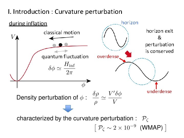
The inflaton field $ϕ$ is fundamentally a quantum field. Its vacuum state is not static but possesses zero-point energy and quantum fluctuations, $δ ϕ$ .
During inflation, the universe undergoes a period of quasi-de Sitter expansion, with a nearly constant Hubble rate, $H$ . The physical wavelength of any perturbation is stretched exponentially: $λ_{phys} (t) = a (t) λ_{comoving}$ .
A key length scale is the Hubble radius, $H^{- 1}$ . Fluctuations begin with wavelengths much smaller than this ( $λ_{phys} ≪ H^{- 1}$ ), where they behave like ordinary quantum fluctuations in flat spacetime.
As inflation proceeds, their wavelength is stretched until it becomes larger than the Hubble radius ( $λ_{phys} > H^{- 1}$ ). This is called horizon exit.
Once a fluctuation is super-Hubble, its endpoints are no longer in causal contact. The fluctuation can no longer oscillate or propagate. It becomes "frozen" into the background spacetime, transitioning from a virtual quantum fluctuation to a real, classical perturbation.

This process is visualized beautifully in the following diagram, which shows how quantum fluctuations in the inflaton field are the origin of all structure.

Origin of Curvature Perturbations During Inflation — This diagram illustrates the core mechanism of this lesson. The inflaton field $\phi$ rolls down its potential $V(\phi)$. Quantum mechanics dictates that its value has a fundamental uncertainty or 'fluctuation' ($\delta\phi$). During inflation, these fluctuations are stretched to scales larger than the Hubble horizon, where they freeze in as classical density perturbations ($\delta\rho$) and curvature perturbations ($\zeta$).

2. Quantizing a Scalar Field in an Expanding Universe

Let's now make this picture rigorous. Your preference for mathematical detail will be well-served here. We will quantize a scalar field in a quasi-de Sitter background. To start, we'll consider a generic, massless "spectator" field $χ$ and then apply our findings to the inflaton itself.

The following reading from Antonio Riotto's lecture notes, "Inflation and the Theory of Cosmological Perturbations," provides the exact derivation we need.

Inflation and the Theory of Cosmological Perturbations

This resource provides the rigorous QFT calculation for a scalar field in a de Sitter background. It's a foundational calculation in modern cosmology.

Please study Section 14.1, 'Quantum fluctuations of a generic massless scalar field during a de Sitter stage' (pages 38-41). Your goal is to understand the mathematical steps that lead to a scale-invariant spectrum. Start with the equation of motion for a Fourier mode \delta\chi_k in an FRW background (Eq. 133). Follow the redefinition of the field to \delta\sigma_k = a \delta\chi_k and the change to conformal time au. Note how this produces the canonical harmonic oscillator equation with a time-dependent potential term, \delta\sigma_k'' + (k^2 - a''/a)\delta\sigma_k = 0 (Eq. 136). Analyze the two asymptotic regimes: the oscillating solution for sub-Hubble modes (k \gg aH) and the 'frozen' solution for super-Hubble modes (k \ll aH). Understand the choice of vacuum state (the Bunch-Davies vacuum), which sets the initial conditions for the mode functions in the sub-Hubble limit. Follow the derivation of the exact solution (Eq. 145) and its super-Hubble limit, which shows that the original field fluctuation \delta\chi_k becomes constant.

Summary of the Calculation

Let's distill the key results from this rigorous derivation.
The equation for a Fourier mode of a massless scalar field in a de Sitter background is:

δ χ ¨_{k} + 3 H δ χ ˙_{k} + \frac{k ^{2}}{a ^{2}} δ χ_{k} = 0

After a canonical transformation, this equation is solved. The crucial result is the amplitude of the mode after it has exited the horizon ( $k ≪ a H$ ):

∣ δ χ_{k} ∣ \approx \frac{H}{2 k ^{3}}

This expression contains profound physics. To see it, we define the power spectrum $P_{χ} (k)$ , which measures the variance of the field fluctuations per logarithmic interval in k-space. It is defined as:

P_{χ} (k) = \frac{k ^{3}}{2 π ^{2}} ⟨ ∣ δ χ_{k} ∣^{2} ⟩

Plugging in our result for $δ χ_{k}$ , we find:

P_{χ} (k) = (\frac{H}{2 π})^{2}

This spectrum is independent of the wavenumber $k$ ! This is the famous scale-invariant spectrum. It means that the amplitude of the frozen fluctuations is the same on all scales. The factor $k^{3}$ in the definition of $P (k)$ is precisely what makes a $1/ k^{3}$ dependence in $⟨ ∣ δ χ_{k} ∣^{2} ⟩$ "scale-invariant".

3. From Inflaton Fluctuations to Curvature Perturbations

We have found the spectrum for a generic spectator field. But the inflaton is special. Because it dictates the energy density of the universe, its fluctuations directly couple to the metric via the Einstein equations:
$δ ϕ ⟹ δ T_{μν} ⟹ δ g_{μν}$
The most intuitive way to understand this connection is through the "time-delay" mechanism.

The following resource provides an elegant, physics-first derivation of this connection.

Lectures on Inflation Introduction

The lecture notes by Leonardo Senatore offer a beautiful physical argument connecting inflaton fluctuations (\delta\phi) to the curvature perturbations (\zeta) we see. This is the crucial conceptual link.

Please read Section 2.3, 'Contact with observation: Part 1' (pages 21-23). Focus on the logic behind Eq. (82) and how it translates a fluctuation in the field, \delta\phi, into a fluctuation in the local amount of expansion, \zeta. The argument distinguishing this from the energy fluctuation (the 'It is the time-delay, stupid!' section) is particularly insightful.

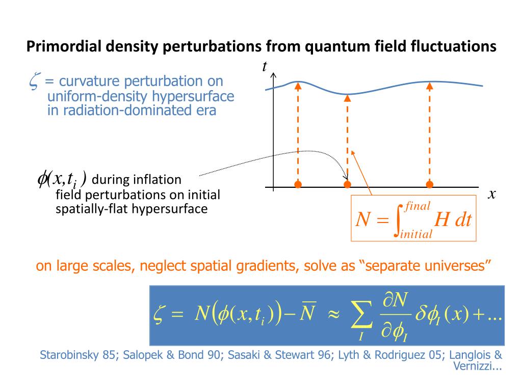
Let's walk through this beautiful argument:

Imagine inflation ends when the field $ϕ$ reaches a specific value, $ϕ_{end}$ .
Now consider a point in space where a quantum fluctuation has given the field a small boost, $δ ϕ$ . At this point, the field will reach $ϕ_{end}$ at a slightly different time. The time delay is $δ t \approx δ ϕ / ϕ ˙_{0}$ , where $ϕ ˙_{0}$ is the classical background velocity of the field.
This time delay means that this particular region of space inflates for a slightly different duration. The number of e-folds of expansion, $N = H t$ , is perturbed by $δ N = H δ t$ .
A perturbation in the number of e-folds corresponds to a perturbation in the local scale factor: $a (x) = a_{0} e^{N_{0} + δ N (x)} = a_{0} e^{N_{0}} (1 + δ N (x) + \dots)$ . The fractional perturbation is $δ a / a = δ N$ .
This local perturbation to the scale factor is precisely the gauge-invariant curvature perturbation, $ζ$ .

So, we have the direct relationship:

ζ = δ N = H δ t = \frac{H}{ϕ ˙ _{0}} δ ϕ

Primordial Density Perturbations from Quantum Field Fluctuations — This diagram from a lecture by David Wands visualizes the time-delay mechanism. A fluctuation in the field value $\phi$ on an initial flat hypersurface is mapped to a fluctuation in the number of e-folds $N$, which becomes the final curvature perturbation $\zeta$ on a uniform density hypersurface after inflation.

Now we can compute the power spectrum of the physical observable, $ζ$ .

P_{ζ} (k) = (\frac{H}{ϕ ˙ _{0}})^{2} P_{δ ϕ} (k)

Using our result $P_{δ ϕ} (k) = (H /2 π)^{2}$ and the slow-roll relation $ϕ ˙_{0}^{2} = 2 M_{P l}^{2} ϵ H^{2}$ , where $ϵ = - H ˙ / H^{2}$ is the slow-roll parameter, we arrive at one of the most important results in cosmology:

P_{ζ} (k) = \frac{H ^{2}}{2 M _{P l}^{2} ϵ H ^{2}} (\frac{H}{2 π})^{2} = \frac{1}{2 ϵ M _{P l}^{2}} (\frac{H}{2 π})^{2}

Since $H$ and $ϵ$ evolve very slowly during inflation, the spectrum is nearly scale-invariant. This small deviation from perfect scale-invariance, called the "tilt," is a key prediction that we will calculate in the next lesson.

4. Classicality and Gaussianity

Two final, crucial points remain. Why do these quantum fluctuations behave like a classical stochastic field in the late universe? And what are their statistical properties?

Quantum-to-Classical Transition: During horizon exit, the state of each mode becomes extremely squeezed. In the phase space of the mode's harmonic oscillator, the uncertainty ellipse is stretched enormously in one direction (field amplitude) and compressed in the other (momentum). A highly squeezed state has a large occupation number and behaves, for all practical purposes, like a classical wave with a well-defined but random amplitude and phase.
Gaussianity: In the simplest models of inflation, the inflaton is a free (or very weakly interacting) field. The action for its fluctuations, $δ ϕ$ , is quadratic. A quantum field theory with a quadratic action is equivalent to a collection of independent harmonic oscillators (one for each Fourier mode). The ground state of a harmonic oscillator is a Gaussian wave function. Therefore, the resulting perturbations $ζ$ are predicted to be drawn from a Gaussian random field. This means their statistical properties are fully described by the two-point correlation function, or its Fourier transform, the power spectrum $P_{ζ} (k)$ .

Test your understanding!

The amplitude of the power spectrum of curvature perturbations is observed to be $P_{ζ} \approx 2 \times 1 0^{- 9}$ . If we assume a slow-roll parameter value of $ϵ \approx 0.01$ , can you use our derived formula for $P_{ζ} (k)$ to estimate the energy scale of inflation, $V^{1/4}$ ? (Recall the Friedmann equation during inflation, $H^{2} \approx V / (3 M_{P l}^{2})$ ).

Show answer

We have the formula $P_{ζ} = \frac{1}{2 ϵ M _{P l}^{2}} (\frac{H}{2 π})^{2}$ . We can rearrange this to solve for $H^{2}$ :
$H^{2} = P_{ζ} \cdot (2 ϵ M_{P l}^{2}) \cdot (4 π^{2})$
Now, using the Friedmann equation $V = 3 M_{P l}^{2} H^{2}$ , we can substitute for $H^{2}$ :
$V = 3 M_{P l}^{2} [P_{ζ} \cdot (2 ϵ M_{P l}^{2}) \cdot (4 π^{2})] = 24 π^{2} ϵ P_{ζ} M_{P l}^{4}$
Plugging in the numbers $ϵ = 0.01$ and $P_{ζ} = 2 \times 1 0^{- 9}$ :
$V \approx 24 π^{2} (0.01) (2 \times 1 0^{- 9}) M_{P l}^{4} \approx 4.7 \times 1 0^{- 9} M_{P l}^{4}$
The energy scale is $V^{1/4}$ :
$V^{1/4} \approx (4.7 \times 1 0^{- 9})^{1/4} M_{P l} \approx (0.0015) M_{P l}$
Given $M_{P l} \approx 2.4 \times 1 0^{18}$ GeV, this gives:
$V^{1/4} \approx 3.6 \times 1 0^{15} GeV$
This is a remarkable result. It shows that the observed amplitude of cosmic perturbations points to an inflationary energy scale that is close to the Grand Unification (GUT) scale, far beyond the reach of any terrestrial particle accelerator.

Conclusion

Today we have unveiled the modern origin story for cosmic structure. We have built a model that traces the largest structures in the universe back to their genesis as microscopic quantum fluctuations.

Key Takeaways:

The origin of primordial perturbations is the quantum vacuum fluctuations of the inflaton field, $δ ϕ$ .
During inflation, these fluctuations are stretched to super-Hubble scales, where they "freeze out" and become classical perturbations.
The fundamental process yields a nearly scale-invariant power spectrum, $P (k) \propto k^{n_{s} - 1}$ with $n_{s} \approx 1$ .
A fluctuation in the field, $δ ϕ$ , creates a time delay in the end of inflation, which in turn generates a curvature perturbation $ζ \approx (H / ϕ ˙_{0}) δ ϕ$ .
The simplest inflationary models predict that these primordial perturbations are Gaussian.
The amplitude of the resulting curvature power spectrum is given by $P_{ζ} = \frac{1}{2 ϵ M _{P l}^{2}} (\frac{H}{2 π})^{2}$ .

Preview of the Next Lesson:

We have derived the fundamental form of the power spectrum. In our next lesson, we will calculate the power spectrum of primordial curvature perturbations generated during inflation in full detail. We will go beyond the leading-order approximation to compute the "spectral tilt" $n_{s}$ , relating it directly to the slow-roll parameters $ϵ$ and $η$ . This will complete our journey from a quantum field theory model to concrete, testable predictions that can be compared with high-precision data from the Cosmic Microwave Background.

Recommended resources