Sachs-Wolfe Effect and CMB Anisotropies

1. Photon Energy Shift in a Perturbed Universe

To begin, we need a general expression for how a photon's energy changes as it propagates from the last scattering surface (LSS) at redshift $z\approx 1100$ to us, the observers, at $z=0$. These photons travel along null geodesics in a universe that is not perfectly homogeneous and isotropic but contains small metric perturbations, which we have been characterizing by the potentials $\Psi$ and $\Phi$.

A full derivation starting from the geodesic equation in a perturbed FRW metric is quite involved, but it is the kind of rigorous foundation your physics background supports. We will begin with the final result of such a derivation.

From the reading, the fractional temperature fluctuation $\Delta T/T$ observed in a particular direction $\mathbf{n}$ on the sky can be expressed as:

Let's carefully dissect this crucial equation. The right-hand side is a sum of all the physical effects that can alter a photon's energy on its long journey:

1. Intrinsic Temperature Fluctuation ($\frac{1}{4}{D}_g^{(r)}$): This term represents the actual temperature variation of the photon-baryon plasma at the point on the last scattering surface where the photon was last scattered. $D_g^{(r)}$ is the gauge-invariant radiation density perturbation.
2. Doppler Effect (${\mathbf{v}}_b\cdot \mathbf{n}$): This is the standard Doppler shift caused by the peculiar velocity ${\mathbf{v}}_b$ of the baryon plasma at the point of emission, relative to the observer.
3. Gravitational Redshift/Blueshift (${\Psi }_{\text{dec}}-{\Psi }_0$): This is the change in gravitational potential energy of the photon as it "climbs out" of the potential well ${\Psi }_{\text{dec}}$ at the last scattering surface and "falls into" our local potential well ${\Psi }_0$ today. For anisotropy calculations, the local term ${\Psi }_0$ is usually neglected as it contributes isotropically. The effect is simply a gravitational redshift from the potential at the emission point.
4. Integrated Sachs-Wolfe (ISW) Effect ($\int (\dot{\Psi }+\dot{\Phi })dt$): This term accounts for the energy shifts a photon experiences as it travels through time-evolving gravitational potentials. If a potential well deepens or shallows while a photon is crossing it, the blueshift from falling in will not exactly cancel the redshift from climbing out.

2. The Ordinary Sachs-Wolfe Effect

The term "Sachs-Wolfe effect" in its most common usage refers to a simplified version of this general formula, valid on very large angular scales. These scales correspond to perturbations that were larger than the causal horizon at the time of decoupling ($k\ll a_{dec}{H}_{dec}$).

On such super-horizon scales:

• Causal physics like acoustic oscillations and peculiar velocities had not had time to take effect. We can therefore neglect the intrinsic acoustic term and the Doppler term. More precisely, for adiabatic perturbations, the intrinsic density fluctuation is directly tied to the potential, as we will see.
• In a matter-dominated universe (a good approximation from decoupling until recently), gravitational potentials on super-horizon scales are constant in time. Therefore, $\dot{\Psi }=\dot{\Phi }=0$, and the Integrated Sachs-Wolfe term vanishes.

Under these assumptions, our master equation simplifies dramatically:

This tells us that the large-scale CMB anisotropies are sourced by just two effects: the intrinsic temperature of the plasma and the gravitational redshift from the potential at the emission point. The magic of the Sachs-Wolfe effect lies in the relationship between these two terms for adiabatic perturbations—the kind predicted by simple inflationary models.

3. The Famous Factor of 1/3

Let's analyze the two competing terms. It might seem that an overdense region (a potential well, with $\Psi <0$) would be hotter and thus appear as a hot spot in the CMB. However, a photon from that region must climb out of the potential well, losing energy and getting redshifted. Which effect wins?

The answer lies in a beautiful physical argument that combines time dilation with the nature of adiabatic perturbations.

Let's walk through the logic presented in the paper:

1. Gravitational Redshift: A photon climbing out of a potential well ${\Psi }_{\text{dec}}$ experiences an energy shift. This effect contributes a term $+{\Psi }_{\text{dec}}$ to the total $\Delta T/T$. Since overdense regions have $\Psi <0$, this corresponds to a redshift (a cold spot).

2. Intrinsic Temperature: For an adiabatic perturbation, all species (photons, baryons, dark matter) are perturbed together. An overdense region can be thought of as a patch of the universe that is slightly "behind" in its expansion and cooling. Due to gravitational time dilation, clocks in a potential well run slower: $\delta t=\Psi t$.
   In the matter-dominated era, the scale factor evolves as $a\propto t^{2/3}$ and the background temperature cools as $T\propto a^{-1}\propto t^{-2/3}$. A region that is "younger" by $\delta t$ will be hotter by:

   $$\frac{\delta T}{T}=-\frac{2}{3}\frac{\delta t}{t}=-\frac{2}{3}\Psi$$

   This is our intrinsic temperature fluctuation term: $\frac{1}{4}{D}_g^{(r)}=\frac{\delta T}{T}=-\frac{2}{3}\Psi$. So, a potential well ($\Psi <0$) is indeed intrinsically hotter.

3. The Sum: Now we combine the two effects:

   $$\frac{\Delta T}{T}=\underset{\text{Intrinsic Temp.}}{\underbrace{\left(-\frac{2}{3}{\Psi }_{\text{dec}}\right)}}+\underset{\text{Grav. Redshift}}{\underbrace{\left({\Psi }_{\text{dec}}\right)}}=\frac{1}{3}{\Psi }_{\text{dec}}$$

This is the celebrated Sachs-Wolfe formula. It reveals a profound fact: the gravitational redshift effect is stronger than the intrinsic temperature effect. Therefore, a large-scale overdensity, corresponding to a potential well with $\Psi <0$, appears as a cold spot on the CMB sky.

This result is derived explicitly from the full perturbation equations in the Durrer notes.

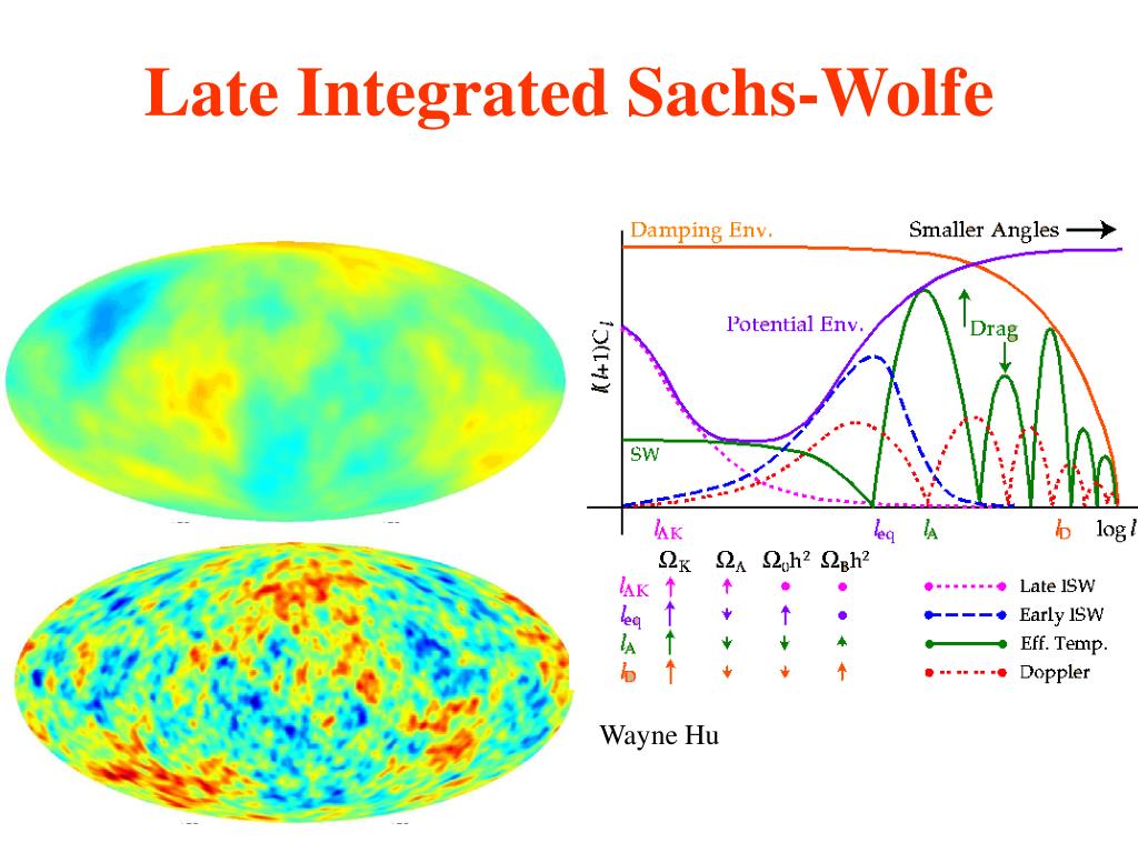
4. The Integrated Sachs-Wolfe (ISW) Effect

We assumed $\dot{\Psi }=0$ to derive the ordinary Sachs-Wolfe effect. This is only true in an Einstein-de Sitter (matter-only, flat) universe. In our actual Universe, this is not quite right at two key epochs:

• Early ISW: Around the time of matter-radiation equality, the Universe was transitioning from being radiation-dominated to matter-dominated. During this transition, potentials decayed, leading to $\dot{\Psi }\ne 0$.
• Late ISW: At late times ($z\lesssim 1$), dark energy began to dominate, causing the cosmic expansion to accelerate. This acceleration also causes gravitational potentials to decay.

When potentials decay ($\dot{\Psi }<0$), photons passing through a potential well gain a net amount of energy. They fall into a deep well, but by the time they climb out, the well has become shallower. This results in a net blueshift. The ISW effect, while generally smaller than the ordinary SW effect, provides a crucial probe of dark energy and the transition from radiation to matter domination.

5. From Potential to Power Spectrum

The Sachs-Wolfe formula provides a direct link between the temperature anisotropies and the primordial gravitational potential. This allows us to translate the statistics of the potential, encoded in its power spectrum $P_{\Psi }(k)$, into the statistics of the CMB temperature map, encoded in its angular power spectrum $C_{\ell }$.

The derivation involves expanding the temperature field in spherical harmonics $Y_{\ell m}$ and relating the coefficients $a_{\ell m}$ to the Fourier modes of the potential $\Psi (\mathbf{k})$.

The key result from this calculation is that the angular power spectrum $C_{\ell }$ due to the Sachs-Wolfe effect is given by an integral over the primordial potential power spectrum:

where $j_{\ell }$ are spherical Bessel functions and $r_{\text{dec}}$ is the comoving distance to the LSS.

For a nearly scale-invariant primordial spectrum, as predicted by inflation, the term in brackets $k^3{P}_{\Psi }(k)$ is approximately constant. The integral can then be evaluated to show that:

This prediction of a flat "plateau" in the angular power spectrum at large scales (low $\ell$) was a landmark success for inflationary cosmology, spectacularly confirmed by the COBE satellite in the early 1990s and measured with incredible precision by WMAP and Planck.

Conclusion

In this lesson, we have forged a direct link between the primordial perturbations from the very early universe and the largest features we see in the Cosmic Microwave Background.

Key Takeaways:

• The temperature anisotropy of a CMB photon is sourced by its intrinsic temperature at last scattering, Doppler shifts, and gravitational potential effects (both at the LSS and along its path).
• On large angular scales, for adiabatic perturbations, the anisotropies are dominated by the Ordinary Sachs-Wolfe effect.
• This effect is a combination of two competing terms: an intrinsic temperature fluctuation ($\Delta T/T=-2/3\Psi$) and a gravitational redshift ($\Delta T/T=+\Psi$).
• The gravitational redshift is stronger, leading to the famous result $\Delta T/T=(1/3)\Psi$. This means large-scale potential wells ($\Psi <0$) appear as cold spots in the CMB.
• For a scale-invariant primordial spectrum, the Sachs-Wolfe effect predicts a nearly flat power spectrum at low multipoles ($\ell (\ell +1)C_{\ell }\approx \text{constant}$), a key feature of the observed CMB.

Preview of the Next Lesson:

We have now completed our deep dive into cosmological perturbation theory, connecting the physics of inflation to two of the most powerful cosmological observables: the large-scale structure of galaxies and the anisotropies in the CMB.

We will now change gears significantly. The next module, "Advanced Topics in Gravity," returns to the fundamental mathematical structure of General Relativity itself. Our first topic will be the 3+1 ADM decomposition of spacetime. This formalism splits spacetime into "space" and "time" and is the foundation for formulating GR as a dynamical theory, essential for numerical relativity (simulating black hole mergers) and canonical quantum gravity.