DAGs: Visualizing Causal Assumptions

1. From Equations to Pictures: Visualizing Causal Structure

In the previous lesson, we saw that an SCM is a collection of equations, like $V_j=f_j(U_j,{\epsilon }_j)$. While these equations provide a complete, quantitative description of a causal system, they can be complex. Often, we first want to reason about the system's qualitative structure: which variables cause which other variables, without specifying the exact mathematical form of the relationship.

This is precisely the role of a Directed Acyclic Graph (DAG). A DAG is the graphical counterpart to an SCM.

As the reading makes clear, the DAG strips away the quantitative details of the functions (f_j) and focuses solely on the causal architecture. An arrow from X to Y in a DAG simply means that X is an argument in the structural equation for Y.

This image provides a perfect illustration of this relationship:

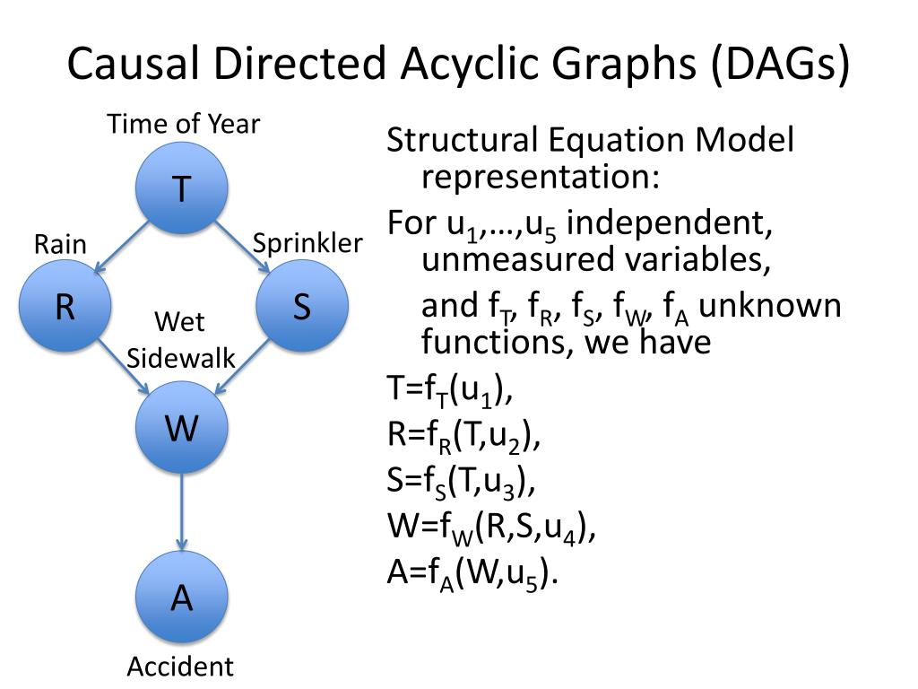
2. The Grammar of DAGs: Encoding Causal Assumptions

To interpret a DAG correctly, we need to understand its basic grammar. A DAG consists of:

• Nodes (or vertices): These represent the variables in our model (e.g., Rain, Sprinkler).
• Arrows (or edges): A directed arrow from node X to node Y represents the assumption that X is a direct cause of Y, relative to the other variables in the model.
• Acyclicity: You can never follow a path of arrows that leads from a node back to itself. This reflects the intuitive assumption that events cannot cause themselves.

The power of a DAG lies not just in the arrows it includes, but also in the ones it leaves out.

This is a crucial philosophical point. A statistical correlation matrix will almost always be dense, with some non-zero correlation between most pairs of variables. A DAG, in contrast, is typically sparse. By omitting an arrow from, say, Sprinkler to Accident, we are making the strong causal claim that the sprinkler does not directly cause an accident, even if they might be statistically correlated. The DAG forces us to be explicit about our causal hypotheses.

3. Why a DAG is Not a Statistical Model

Your background in statistics and probability theory makes you familiar with graphical models that represent statistical dependencies, like Bayesian networks. It's vital to distinguish these from DAGs used for causal inference.

A Bayesian network is a representation of a joint probability distribution. It tells you about conditional dependencies—which variables become independent when you know the value of another. A causal DAG does more: it makes claims about what happens when you intervene on the system.

Let's hear Judea Pearl make this distinction himself.

Pearl's key idea is that the causal assumptions encoded in a DAG are extra-statistical. They cannot be derived from the data alone. We need to bring in outside knowledge or theory about the data-generating process.

The classic example illustrating this is Simpson's Paradox.

This example makes it clear: the statistical information P(Recovery|Drug, Gender) is identical to P(Recovery|Drug, BP). But the causal structures are different.

• Gender is a common cause of Drug (treatment choice) and Recovery. This is a confounding path.
• Blood Pressure is a common effect of the Drug and an underlying illness that also affects Recovery. This is a collider path, a concept we will explore next.

The DAG makes these different causal stories explicit, telling us how to interpret the same statistical patterns.

4. Reading the Causal Story: Paths in a DAG

A DAG tells a causal story through its paths. A path is any sequence of connected nodes, regardless of arrow direction. The way arrows are oriented along a path determines how statistical association flows between variables. Understanding this is the key to interpreting a DAG.

Let's summarize the key ideas from the video:

• Causal Path: A directed path X → ... → Y. This is how a change in X can cause a change in Y. This path is naturally open.
• Confounding Path (Backdoor): A path like X ← C → Y. Here, C is a common cause. This path creates a non-causal statistical association between X and Y because when C varies, X and Y vary together. This path is naturally open, but is closed by conditioning on C.
• Collider Path: A path like X → Z ← Y. Here, Z is a common effect (a "collider"). This path does not create an association between X and Y. It is naturally closed. However, if we condition on the collider Z, we open the path and can create a spurious statistical association between X and Y.

Your experience as a social researcher on relationships provides fertile ground for thinking about these structures. For instance, in polyamorous networks, a person's happiness (Z) might be a collider, influenced by the quality of their relationship with partner X and partner Y. In the general population, the quality of these two relationships might be independent. But if you were to study only very happy people (conditioning on the collider Z), you might find a spurious negative correlation: given high happiness, a great relationship with X might 'explain away' the need for a great relationship with Y.

Conclusion

In this lesson, we have transitioned from the abstract equations of SCMs to the intuitive, qualitative language of Directed Acyclic Graphs.

Key Takeaways:

• DAGs as Qualitative Models: A DAG is the graphical representation of an SCM's structure, showing the presence and, crucially, the absence of direct causal relationships.
• Distinct from Statistical Models: A DAG is not a model of correlations; it is a model of hypothesized causal mechanisms. It contains extra-statistical information that is essential for causal inference, as demonstrated by Simpson's Paradox.
• The Language of Paths: The causal story in a DAG is read through its paths. Causal paths, confounding paths, and collider paths have different properties that determine how statistical association is transmitted or blocked between variables.
• Conditioning's Dual Role: Conditioning on a variable can either block a confounding path (removing bias) or open a collider path (introducing bias). A DAG makes it possible to distinguish between these two cases.

In our next lesson, we will focus on the second rung of the Ladder of Causation: intervention. We will formally define the do-operator and explore why the distinction between seeing, P(Y|X), and doing, P(Y|do(X)), is so philosophically fundamental to this entire framework.