The do-operator and the Philosophy of Causal Inference

1. The Leap from Seeing to Doing

In your work as a statistician, you are an expert at modeling the world as you find it. You can describe the probability of an outcome $Y$ given that you have observed a condition $X$. This is the world of association, the first rung of the causal ladder. However, to ask causal questions—"Does this treatment work?", "What is the effect of this policy?"—we need a language to describe what happens when we actively change the world.

Judea Pearl argues that this requires a conceptual and mathematical leap that traditional statistics, built on symmetric equations, cannot make.

As Pearl explains, each level of this ladder requires a different kind of information and answers a different class of questions. Today, we are focused on formalizing the logic of the second level: Intervention.

2. The do-operator: A Language for Intervention

The core distinction we need to make is between seeing and doing.

• Seeing: We observe that a variable $X$ happens to have a value $x$. We then update our beliefs about another variable $Y$. This is a standard conditional probability, written as $P(Y|X=x)$. It is about passive observation.
• Doing: We force the variable $X$ to take the value $x$, regardless of what its natural causes would have dictated. We then observe the resulting state of $Y$. This is an intervention, and it's written using Pearl's do-operator: $P(Y|\text{do}(X=x))$.

As the article makes clear, $P(Y|X)$ is for prediction or diagnosis, while $P(Y|\text{do}(X))$ is for control or decision-making. For instance, in your research on relationships, observing that people who communicate frequently (X) report high relationship satisfaction (Y) gives you $P(Y|X)$. This is useful for predicting satisfaction. But if you want to design an intervention to improve satisfaction, you need to know the effect of making people communicate more, which is $P(Y|\text{do}(X))$. These two quantities may not be the same, especially if, for example, a third factor like 'shared life goals' causes both frequent communication and high satisfaction.

3. Visualizing the Intervention: A "Surgery" on the Model

How do we conceptualize this do() operation? In the previous lesson, we established that a DAG represents a causal model. An intervention, then, is a modification—a "surgery"—on that model.

When we intervene to set $X=x$, we are severing the natural causal pathways that lead to $X$. The value of $X$ is no longer determined by its parents in the graph; it is determined by our external force.

This image shows the effect of this surgery on the sprinkler system DAG we've seen before.

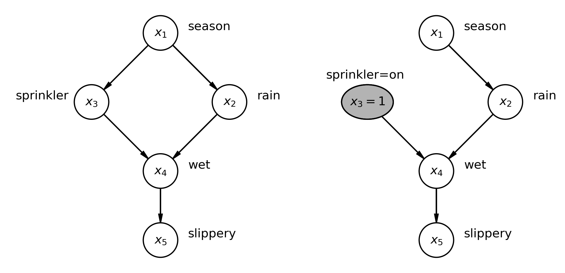
This "graph surgery" is the graphical representation of the do-operator.

Another way to visualize the difference is to think about populations. Conditioning on $X=x$ means we are zooming in on a sub-population that already has this characteristic. Intervening with do(X=x) means we are creating a new hypothetical population where everyone has been forced to have this characteristic.

4. Why the Distinction is Philosophically Fundamental

This distinction isn't just a technical nicety; it's the very heart of causal reasoning. Conflating $P(Y|X)$ with $P(Y|\text{do}(X))$ is the source of countless fallacies and poor decisions. Formally, we can define confounding as the situation where the observational and interventional distributions are not equal:

$P(Y|X=x)\ne P(Y|\text{do}(X=x))$

The most famous example of this is Simpson's Paradox, where the observational data seems to give one answer, while the causal question demands another. Let's see how the do-operator resolves this.

As the example demonstrates, the observational quantity $P(\text{Recovery}|\text{Drug}=1)$ was approximately 0.78, while $P(\text{Recovery}|\text{Drug}=0)$ was 0.83, suggesting the drug is harmful. However, calculating the causal effect via the do-operator yielded $P(\text{Recovery}|\text{do}(\text{Drug}=1))\approx 0.832$ and $P(\text{Recovery}|\text{do}(\text{Drug}=0))\approx 0.782$.

The do-operator forces us to confront the causal question directly: "What would happen if we force everyone to take the drug?" To answer this, we must use our causal model (the DAG) to block the non-causal "backdoor" path Drug ← Sex → Recovery. The distinction between seeing and doing is the difference between a misleading correlation and a life-saving causal conclusion.

5. From Concept to Calculation: The Idea of Identification

You might be asking: if $P(Y|\text{do}(X))$ describes a hypothetical world, how can we ever calculate it from real-world, observational data? This is the central challenge of causal inference.

The process of translating a causal quantity (with a do-operator) into a purely statistical quantity (without one) is called identification. This is possible if and only if our causal model (the DAG) provides enough assumptions to isolate the causal effect from the statistical noise of confounding.

The adjustment formula we saw in the Simpson's Paradox example is one tool for identification. The complete set of rules for this translation is known as the do-calculus. For our purposes, it's most important to grasp the philosophical point: we can only answer "what if I do?" questions from "what if I see?" data if we are willing to posit a causal theory that connects them. Data alone is not enough.

Conclusion

Today we have formalized the crucial step from observation to intervention. This distinction is the bedrock upon which all of causal inference is built.

Key Takeaways:

• Seeing vs. Doing: Observational probability, $P(Y|X)$, describes our updated belief about $Y$ after seeing $X$. Interventional probability, $P(Y|\text{do}(X))$, describes the distribution of $Y$ in a world where we have forced $X$ to a certain value.
• The do-operator as "Surgery": An intervention do(X=x) is modeled as a "surgery" on the causal DAG, where all arrows pointing into $X$ are cut.
• Philosophical Importance: The distinction is fundamental because it separates correlation from causation. Confounding exists precisely when seeing is not the same as doing ($P(Y|X)\ne P(Y|\text{do}(X))$). This allows us to resolve paradoxes like Simpson's and make correct decisions.
• Identification: The goal of causal inference is often to identify an interventional quantity, expressing it in terms of observational data, which is made possible by the assumptions encoded in a causal model.

In our previous lessons, we built up the language of causal models and interventions. We have now reached the top two rungs of the ladder. In our next lesson, we will ascend to the final, most powerful level: Counterfactuals. We will explore how SCMs provide the formal language for asking "what if?" questions about past events that did not happen.