Enhancing Charts with Titles, Labels, and Annotations

1. The Customization Hub: Titles, Axes, and Colors

Once a chart is created in Google Sheets, most of your customization work will happen in the Chart editor pane, under the Customize tab. The key to effective customization is to ensure every element on the chart serves a purpose and adds to the clarity of the message.

The main elements you'll want to control are:

• Chart & Axis Titles: These tell your audience what they are looking at. A chart without a title is like a book without a cover.
• Series: This refers to your actual data (the bars, lines, or pie slices). Changing colors can help draw attention or align with a client's brand.
• Legend: The key that explains what each color or symbol represents.
• Gridlines & Ticks: These help the viewer trace data points back to the axes.

The following video provides a great walkthrough of the "Customize" tab in Google Sheets. It will help you get familiar with where to find these essential options.

The Importance of Axis Titles

While the video focused on the main chart title, adding titles to your axes is just as important. An axis with numbers but no label forces the reader to guess what those numbers mean. Is it dollars, units sold, or something else? You must eliminate this ambiguity.

Although the following video uses Excel, it perfectly explains the thought process behind adding axis titles for clarity. The principle is identical in Google Sheets.

2. Adding Clarity with Data Labels and Annotations

Titles and colors set the stage, but data labels and annotations deliver the specific insights. They point directly to the numbers and stories in your data.

Data Labels

Data labels display the exact value of a data point directly on the chart (e.g., on top of a bar or next to a point on a line). This saves your audience from having to estimate values by looking at the gridlines.

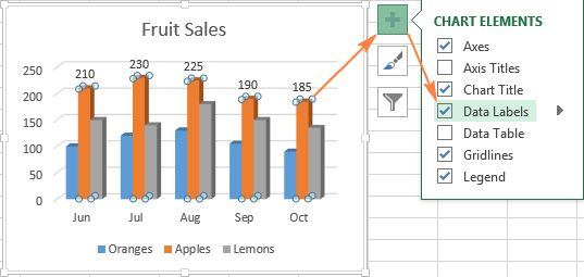
You can easily add these in Google Sheets. The following guide from Google's official help center shows you how.

A pro-tip for clean, professional charts is to use direct labeling where possible. Instead of relying on a separate legend, you can label the data series itself. This reduces the mental effort for the reader.

In Google Sheets, you can achieve this by adding a data label to just the last point of a line chart and editing the label text to be the series name.

Annotations (Notes)

Sometimes, you need to explain why a certain data point is interesting. An annotation is a small note on the chart that provides context. For example, you could add a note to a sales chart that says "New marketing campaign launched" to explain a sudden spike.

The Google Help article you just reviewed also explains how to add these notes. It involves adding a new column in your source data for the note text.

3. Hands-On Practice

It's time to apply these techniques. Please open the practice workbook you used in the previous lesson, which should contain the charts you created. We will focus on improving the line chart showing monthly sales trends.

Follow these steps to transform your basic chart into a professional one:

1. Select your line chart. Double-click it to open the Chart editor pane.
2. Add Titles:
   • Go to the Customize tab.
   • Click on Chart & axis titles.
   • Change the Chart title to something more descriptive, like "2023 Monthly Sales Trend".
   • Change the Title text for the Vertical axis title to "Total Sales (USD)".
3. Add Data Labels:
   • In the Customize tab, go to Series.
   • Check the box for Data labels. This will add labels to every point.
   • To make it cleaner, let's only highlight the highest month. First, uncheck Data labels to remove them all. Then, find the highest point on your chart, and double-click just that single data point. The Chart editor should now show you are formatting only that point. Now check Data labels again. The label should appear for only that single point.
4. Add an Annotation:
   • Go to the pivot table that is the source for your chart.
   • Find the month with the highest sales (e.g., November or December).
   • In the spreadsheet column right next to your pivot table's sales figures, type a note in the cell corresponding to that month. For example: "Start of Holiday Shopping Season".
   • Now, double-click your chart. In the Setup tab of the Chart editor, adjust your Data range to include this new column with your note. A small annotation marker should appear on the chart. Note: If this doesn't work easily with the pivot table, you can copy the pivot table data and paste it as values into a new area, then add the notes column there and create the chart from this new static data.

Once you've finished, your chart should look much more informative and professional than the default version.

Conclusion

You've now learned the essential skills for turning a basic chart into a powerful tool for communication. A well-customized chart not only looks more professional but also guides your audience to the most important insights, preventing confusion and making your findings more impactful.

Here are the key takeaways from this lesson:

• The Customize tab in the Google Sheets Chart editor is your central hub for all formatting.
• Clear titles for the chart and its axes are non-negotiable; they provide essential context.
• Data labels show exact values, while annotations explain the "why" behind the data.
• Aim for clarity above all. A simple, well-labeled chart is always better than a complicated, confusing one.

In our next lesson, you will learn how to take your finished chart and write a concise summary that interprets the data and highlights the key takeaways for a client. This is the final step in packaging your analysis for a report.