Introduction
In our last lesson, we mastered conditional logic with IF, AND, and OR, which allowed you to create new data based on rules within the same row. You learned to flag invoices as "Urgent" or "High Value," making your spreadsheet more intelligent. Now, we'll address a different, but equally common, challenge in data research: combining information from separate tables.
Imagine you have one list of invoices and another list of client details. How do you pull the client's industry or location into your invoice sheet without manually copying and pasting? This lesson introduces VLOOKUP, a cornerstone function for exactly this task. You will learn how to use VLOOKUP to search for a value in one table and retrieve a corresponding piece of data from another. This skill is essential for enriching your datasets, a fundamental activity in data research.
Understanding VLOOKUP: Your Data Librarian
At its core, VLOOKUP (which stands for "Vertical Lookup") acts like a librarian for your spreadsheet. You give it something to look for (like a book title or an order number), tell it which library section to search in (a table of data), and specify what piece of information you want back (like the author's name or the order status).
The function always searches vertically down the first column of the table you specify to find a match. Once it finds the match, it moves horizontally to the right to retrieve the information from the column you've requested.
To get a formal introduction to the VLOOKUP function and its components, let's turn to a well-structured guide.
VLOOKUP in Google Sheets with formula examples - Ablebits.com
This article from Ablebits.com provides a fantastic breakdown of the VLOOKUP syntax with a clear, annotated diagram.
Please read the first section, "Google Sheets VLOOKUP - syntax and usage". Focus on understanding the four arguments: search_key, range, index, and is_sorted. The diagram at the end of this section is particularly helpful for visualizing how these pieces fit together.
The VLOOKUP Formula and Its Arguments
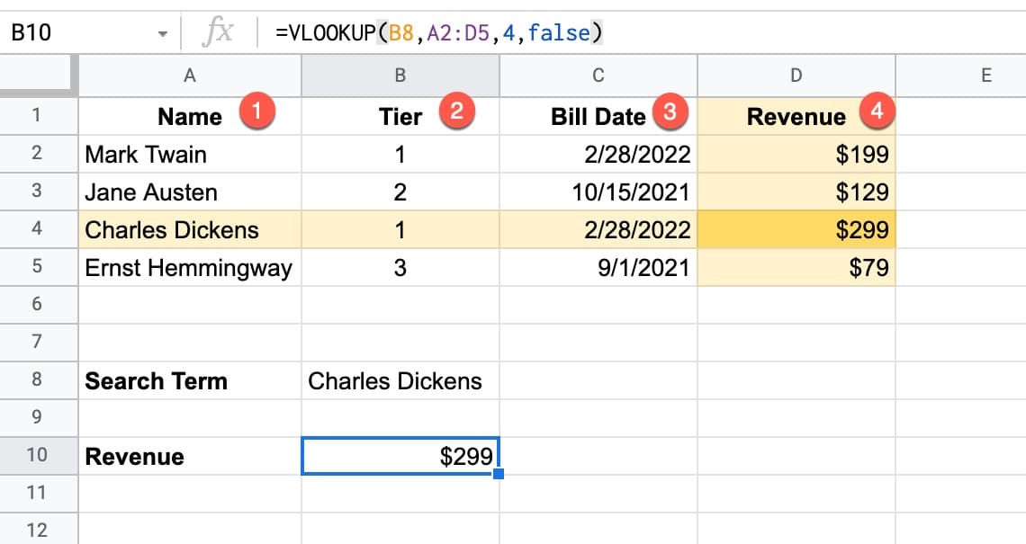
As you just read, the syntax for VLOOKUP is:=VLOOKUP(search_key, range, index, is_sorted)
Let's quickly recap and visualize these components:
search_key(orlookup_value): The piece of information you already have. This is what you're "looking up." In the image below, it's the specific animal name, "Lion".range(ortable_array): The entire table of data where you'll search for thesearch_keyand find the return value. Critically, thesearch_keymust be in the first column of this range.index(orcol_index_num): The column number within yourrangethat contains the information you want to get back. The count starts with 1 for the first column.is_sorted: ATRUE/FALSEvalue that tells Sheets whether your lookup column is sorted. For data research where you need exact matches, this will almost always beFALSE.

The Most Important Argument: is_sorted (FALSE)
The is_sorted argument is crucial. When you set it to FALSE, you are telling VLOOKUP to find an exact match. If it cannot find the exact search_key, it will return an #N/A error. This is exactly what you want for data research because it tells you definitively that the item wasn't found.
If you set it to TRUE (or omit it, as TRUE is the default), VLOOKUP will look for an approximate match. This can lead to incorrect data being returned if your lookup column isn't perfectly sorted, which is a risky and unreliable approach for most data research tasks.
To see a clear demonstration of why FALSE is the safer and more reliable choice, watch this short video.
How to use VLOOKUP in Google Sheets
This clip from Teacher's Tech provides a direct comparison between using TRUE (approximate match) and FALSE (exact match) in a VLOOKUP.
Watch from the beginning of this section. Pay close attention to what happens when the formula uses TRUE for a value that doesn't exist versus what happens when it uses FALSE. Notice how FALSE returns an error, correctly indicating the value is missing.
The key takeaway is simple: when you need to be sure you have the right data for the right item, always use FALSE for an exact match.
Practical Exercise: Enriching Your Invoice Data
Let's apply VLOOKUP to the My Freelance Invoices spreadsheet you've been working on. Imagine you have a separate list that categorizes your clients by industry. Your goal is to add this "Industry" information to your main invoice sheet.
Part 1: Create the Lookup Table
- Open your
My Freelance Invoicesspreadsheet. - Create a new sheet by clicking the
+icon at the bottom-left. - Rename this new sheet to "Client Details".
- In this "Client Details" sheet, set up a small table as follows:
- In cell A1, type Client Name.
- In cell B1, type Industry.
- In the rows below, list a few clients from your main invoice sheet and assign them an industry. For example:
| Client Name | Industry |
|---|---|
| Sunshine Navigations | Logistics |
| Quantum Leap Inc. | Technology |
| Silver Screen Prod. | Media |
| Apex Solutions | Consulting |
Part 2: Use VLOOKUP to Pull in the Data
- Go back to your main invoice sheet (likely named "Sheet1" or the name you gave it).
- Add a new column header in cell K1 (or the next available column) called "Industry".
- In cell K2, you'll write your
VLOOKUPformula. Let's build it step-by-step:- Start the formula:
=VLOOKUP( search_key: The value we want to look up is the client's name for this row, which is in cell B2. So, typeB2,.range: This is our new table in the "Client Details" sheet. Go to the "Client Details" sheet and select the range of your data, for example,A2:B5. Your formula bar will automatically update to'Client Details'!A2:B5.- Crucial Step: We need to "lock" this range so it doesn't shift when we drag the formula down. Press the F4 key (or add
$signs manually) to change the range to$'Client Details'!$A$2:$B$5.
- Crucial Step: We need to "lock" this range so it doesn't shift when we drag the formula down. Press the F4 key (or add
index: We want to return the "Industry," which is the 2nd column in our selected range (A2:B5). So, type,2,.is_sorted: We need an exact match. So, typeFALSE).
- Start the formula:
- Your final formula should look like this:
=VLOOKUP(B2, 'Client Details'!$A$2:$B$5, 2, FALSE) - Press Enter. The correct industry should appear for the client in that row.
- Drag the fill handle (the small blue circle) down the "Industry" column to apply the formula to all your invoices.
You have successfully enriched your dataset by pulling in related information from another table, a task you will perform constantly as a data researcher.
Conclusion
Today, you've added one of the most practical and powerful functions in any spreadsheet user's toolkit. VLOOKUP bridges the gap between different sets of data, allowing you to build richer, more connected information systems without tedious manual work.
Here are your key takeaways:
VLOOKUPis used to search for a value in the first column of a table and return a corresponding value from another column in that same row.- The function requires four arguments:
search_key,range,index, andis_sorted. - For data research tasks requiring accuracy, the
is_sortedargument should always be set toFALSEto ensure an exact match. - Using absolute references (
$) for therangeis essential when copying aVLOOKUPformula down a column.
In our next lesson, we will focus on cleaning and standardizing data with text functions like TRIM, PROPER, and CONCATENATE. Now that you can pull data together with VLOOKUP, the next logical step is to ensure that data is clean, consistent, and ready for analysis.