Essential Functions: SUM, COUNT, AVERAGE

In our last session, you took the first essential steps in organizing data by creating and formatting an invoice tracker. You now have a clean, structured table with raw numbers. This lesson will show you how to bring that data to life by performing calculations. For a data researcher, this is where the real work begins: transforming lists of numbers into actionable insights for your freelance clients.

Today, you will learn to use some of the most fundamental functions in Google Sheets: SUM, COUNT, and AVERAGE. By the end of this lesson, you'll be able to calculate total revenue, count the number of projects, and find the average project value in your invoice tracker.

Formulas vs. Functions

Before we dive in, it's important to understand a key distinction. In spreadsheets, we perform all calculations using formulas, which always begin with an equals sign (=). A formula can be a simple arithmetic operation, like =10 * 5.

However, for more complex tasks, we use functions, which are pre-built formulas that perform a specific calculation. For example, instead of typing =D4+D5+D6+D7, you can simply use the SUM function: =SUM(D4:D7). Functions save time and reduce errors.

This video provides an excellent explanation of the difference and shows how to build both simple formulas and use your first functions.

Google Sheets for Beginners - The Complete Course

This tutorial from Technology for Teachers and Students clearly demonstrates the building blocks of spreadsheet calculations.

Please watch two key segments: Start with the section on creating formulas from this part. Pay close attention to how every formula starts with = and how you can click on cells to reference them instead of typing their values. This makes your formulas dynamic. Next, watch the introduction to functions from the next segment. This will introduce the SUM function and show you the basic syntax, which applies to most functions you'll learn.

The Core Functions: SUM, AVERAGE, and COUNT

Now that you understand the basic concept, let's focus on three functions that are essential for any data analysis task.

SUM: Adds up all the numbers in a range of cells.
COUNT: Counts how many cells in a range contain numbers.
AVERAGE: Calculates the average of the numbers in a range.

The following guide provides a clear, step-by-step walkthrough for using these functions.

How to use Google Sheets: The Complete Beginner's Guide

This guide by Ben Collins is a great reference for the most common functions.

Read the section titled Starting with functions. Follow the instructions for COUNT, SUM, and AVERAGE. Notice the syntax: the function name is followed by parentheses containing the cell range you want to analyze (e.g., D4:D7).

As you saw in the guide, the process is straightforward:

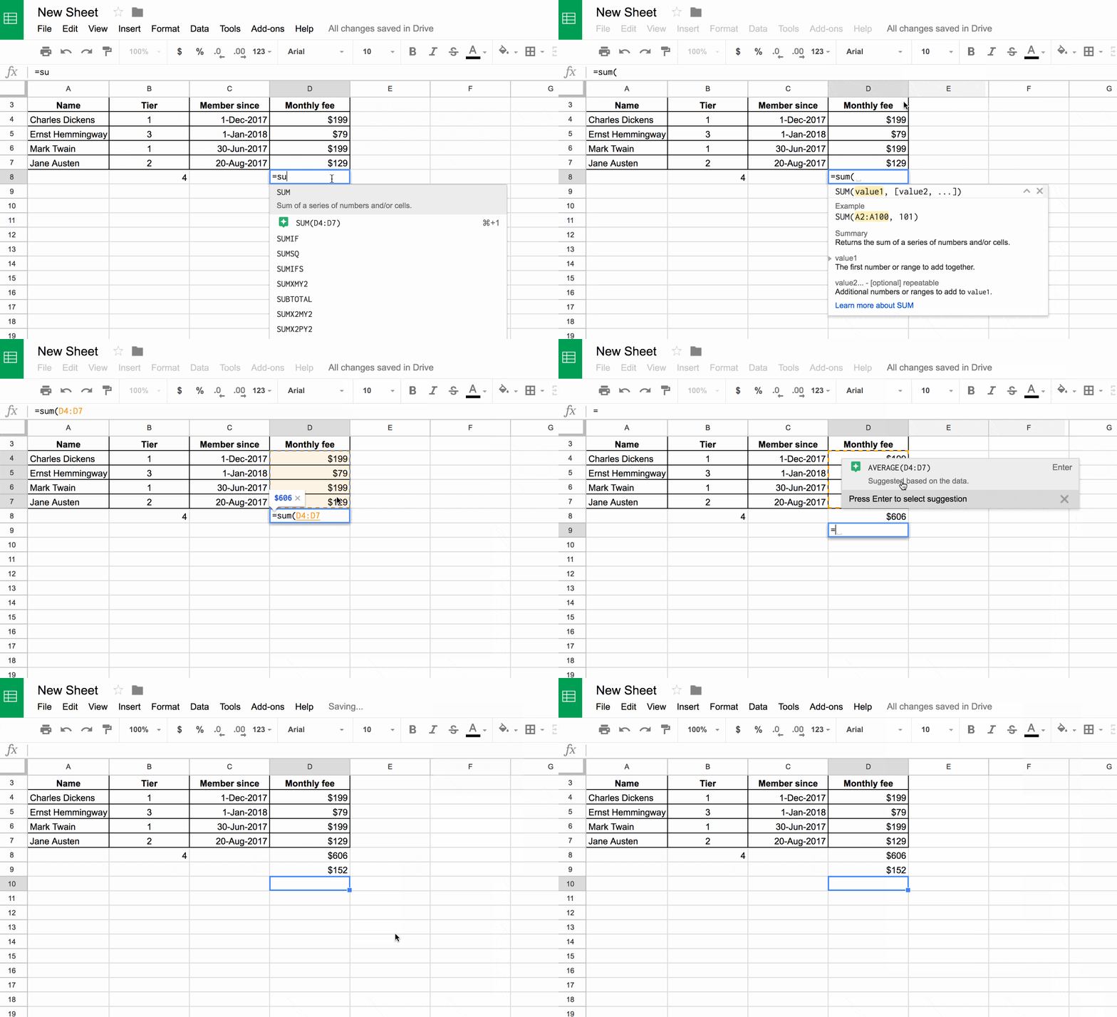
This animation shows the process of typing a function like `=SUM(` and then highlighting the desired cell range with the mouse.

A useful variation is the COUNTA function. While COUNT only counts cells with numbers, COUNTA counts any cell that is not empty, including those with text. This is useful for counting things like the number of clients or projects listed.

A Quick Analysis Shortcut

Sometimes you need a quick calculation without adding a new formula to your sheet. Google Sheets has a built-in summary feature for this. If you highlight a range of cells containing numbers, a small box appears in the bottom-right corner showing the SUM, AVERAGE, COUNT, and more. This is a great way to check your work or get a fast insight.

The quick summary bar provides instant calculations for any selected range, which is perfect for rapid data exploration.

Expanding Your Toolkit: MIN and MAX

Two other incredibly useful functions are MIN and MAX. As their names suggest, they find the minimum and maximum values in a range, respectively. These are great for quickly identifying the highest and lowest invoice amounts, the earliest or latest dates, or any other extreme values in your data.

This short video demonstrates how to use them.

Google Sheets Formulas Tutorial

This clip from Kevin Stratvert's "Google Sheets Formulas Tutorial" provides a quick and clear example of using MIN and MAX.

Watch the segment from using MIN and MAX. Notice that the syntax is identical to the other functions you've learned: =MAX(range) and =MIN(range).

Practical Exercise: Analyze Your Invoice Tracker

It's time to apply what you've learned to the My Freelance Invoices sheet you created in the last lesson. You will add a summary section to get a high-level overview of your freelance business.

Open your sheet: Open the My Freelance Invoices spreadsheet. If you added more sample data, that's great! If not, the two rows from the last lesson will work fine.
Create a Summary Area: In a clear space below or to the side of your main table (e.g., starting in cell A8), create the following labels in a column:
- Total Revenue
- Number of Invoices
- Average Invoice Value
- Highest Invoice
- Lowest Invoice
Calculate the Metrics: In the cells directly to the right of your new labels, enter the formulas to calculate each metric. Assume your invoice amounts are in column D.
- For Total Revenue, use the SUM function on your Amount (USD) column. The formula will look something like =SUM(D4:D5).
- For Number of Invoices, use the COUNT function on the same Amount (USD) column: =COUNT(D4:D5).
- For Average Invoice Value, use the AVERAGE function: =AVERAGE(D4:D5).
- For Highest Invoice, use the MAX function: =MAX(D4:D5).
- For Lowest Invoice, use the MIN function: =MIN(D4:D5).

After completing these steps, you will have a dynamic summary that automatically updates as you add new invoices to your tracker. This is the power of spreadsheet formulas!

Conclusion

You've successfully made the leap from organizing data to analyzing it. This is a fundamental skill for any data researcher. By summarizing large datasets into a few key numbers, you provide immediate value and clarity.

Here are the key takeaways from this lesson:

All calculations start with an equals sign (=).
Functions like SUM, COUNT, and AVERAGE automate common calculations on a range of cells.
The basic syntax is consistent: =FUNCTION(range).
Functions such as MIN and MAX help you quickly find the extremes in your data.
The quick summary bar is an efficient tool for on-the-fly analysis without writing formulas.

Now that you can calculate key metrics, you might wonder how to make important data stand out automatically—for instance, highlighting invoices over a certain amount or those that are due soon. In our next lesson, we will explore conditional formatting, a powerful tool that changes a cell's appearance based on the data it contains.