Welcome back! In our first lesson, you learned the essentials of navigating Google Sheets, including how to create, name, and open your workbooks. This gave you the keys to the workshop. Now, it's time to start building.
This lesson focuses on the core activity of any data project: entering and formatting data. As a data researcher, your primary role is to bring structure to information. Clean, well-organized data is not just easier to read; it's the foundation for accurate analysis and professional-looking reports for your clients. By the end of this session, you will be able to enter text, numbers, and dates into a spreadsheet and format them for clarity and impact.
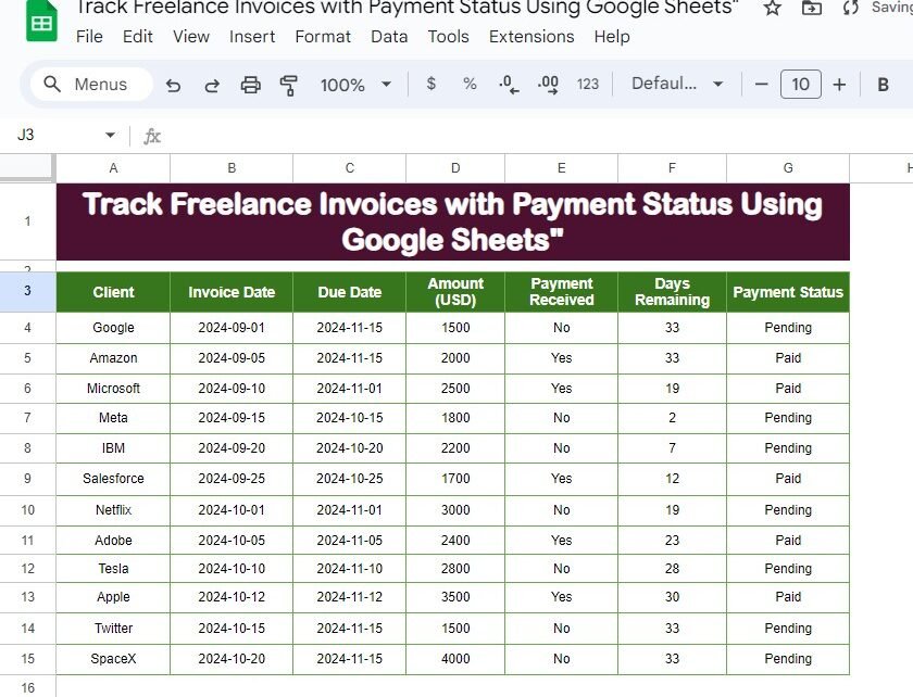
To make this practical, we'll work towards building a simple but powerful tool that every freelancer needs: an invoice tracker.
The Fundamentals of Data Entry
Before we can format data, we need to get it into the cells. The process is simple, but a few key habits can make you much more efficient. The basic workflow is to click on a cell, type your data, and then move to the next cell.
- Pressing Enter commits the data and moves the active cell down one row. This is useful for entering data in a single column.
- Pressing Tab commits the data and moves the active cell right one column. This is perfect for filling out a single row of information, like a client record.
For a quick refresher and some clear, practical advice on entering different types of data, please review the following guide.
How to Enter Data in Google Sheets: A Practical Guide
This guide from How-To Sheets provides excellent, straightforward tips for data entry.
Focus on these two parts: First, read the steps under the heading "Select a starting cell...". This covers the basic mechanics of using your keyboard to navigate efficiently. Then, read the section Entering different data types. Pay attention to the advice on keeping text consistent and entering numbers without extra formatting.
From Raw Data to a Structured Table
Simply typing data into cells isn't enough. For a sheet to be useful, it needs structure. This usually starts with creating clear headers for your columns.
Let's watch a short video that demonstrates how to enter headers and then adjust the column widths so all your text is visible. This is one of the most common formatting tasks you'll perform.
Beginners Google Sheets Tutorial - Lesson 1
This clip from the "Beginners Google Sheets Tutorial" by Teacher's Tech shows the first steps in structuring a dataset.
Watch the segment from creating headings and adjusting columns. Notice the two methods for changing column width: Manually dragging the border between column letters. Double-clicking the border to automatically fit the content.
The double-click method is a significant time-saver, especially when you have many columns to adjust.
Now, let's add a title to our sheet. A good title explains what the data is about. To make it stand out, we can make it span across all the columns of our table by merging cells. The same video shows how to do this, and also how to apply basic text formatting like bolding and alignment.
Beginners Google Sheets Tutorial - Lesson 1
Continuing with the Teacher's Tech tutorial, let's see how to create a professional-looking title.
Watch from inserting a row for a title. This part covers: Inserting a new row above your existing data. Selecting a range of cells and using the Merge cells button. Using the Horizontal align button to center the title text. Then, continue watching from the next brief section to see how to make the text bold and change its font size.
Enhancing Readability with Formatting
With the basic structure in place, we can use color, borders, and number formatting to make the data easy to interpret. These visual cues help distinguish headers from data and draw attention to important information.
Let's watch a few more short clips that demonstrate how to:
- Apply background colors to headers.
- Add borders to create a distinct table.
- Format numbers as currency.
Beginners Google Sheets Tutorial - Lesson 1
These final clips from the Teacher's Tech tutorial cover key visual formatting options.
Please watch the following segments: Color and Font: See how to use the Fill color and Text color tools to make your headers stand out. Adding Borders: Learn how to use the Borders tool to outline your data table. Formatting Numbers: This shows how to apply Currency format and adjust decimal places, which is essential for financial data.
Practical Exercise: Build Your Invoice Tracker
Now it's time to apply everything you've learned. You will create the invoice tracker shown at the beginning of the lesson.
- Create and Name: Open a new spreadsheet using the
sheets.newshortcut and name itMy Freelance Invoices. - Enter Title and Headers:
- In cell
A1, type the title:Track Freelance Invoices with Payment Status Using Google Sheets. - In row
3, starting from cellA3, type the following headers, using theTabkey to move across the row:
Client,Invoice Date,Due Date,Amount (USD),Payment Received,Days Remaining,Payment Status.
- In cell
- Enter Data:
- Enter the first two rows of data as shown in the image. For the dates, you can type them as
2024-09-01. Google Sheets will recognize them as dates. Don't worry about the "Days Remaining" column for now; we'll learn how to calculate that later.
- Enter the first two rows of data as shown in the image. For the dates, you can type them as
| Client | Invoice Date | Due Date | Amount (USD) | Payment Received | Payment Status |
|---|---|---|---|---|---|
| 2024-09-01 | 2024-11-15 | 1500 | No | Pending | |
| Amazon | 2024-09-05 | 2024-11-01 | 2000 | Yes | Paid |
- Apply Formatting:
- Title: Select cells
A1throughG1. Click the Merge cells button, then set the Horizontal align to Center. Make the title text Bold. - Headers: Select the header row (
A3:G3). Make the text Bold. Choose a dark Fill color and a light Text color for contrast (e.g., dark green with white text). - Column Widths: Double-click the border between each column header (between A and B, B and C, etc.) to automatically resize them to fit the content.
- Number Formatting: Select the
Amount (USD)column data (D4:D5). Click the Format as currency ($) button. If it adds decimals, use the Decrease decimal places button twice to remove them. - Alignment: Select the data in the
Payment Receivedcolumn (E4:E5) and use the Horizontal align button to center the text. - Borders: Select your entire table, from
A3toG5. Click the Borders button and choose All borders.
- Title: Select cells
When you're finished, your sheet should look very similar to the target image.
Conclusion
Congratulations! You've moved beyond just navigating a spreadsheet and have started to shape it into a useful, professional document. This is a critical skill for any freelance data researcher, as presenting clear and organized data is just as important as gathering it.
Here are the key takeaways from this lesson:
- You can enter data efficiently using the Enter (down) and Tab (right) keys.
- Data comes in different types, like text, numbers, and dates, and Google Sheets can recognize them.
- Formatting tools are used to improve readability:
- Adjusting column widths ensures all text is visible.
- Merging cells is great for creating titles.
- Bold, fill color, and text color create visual hierarchy.
- Borders help define your data table.
- Number formats (like currency) make numerical data meaningful.
You now have a sheet containing numerical data. In our next lesson, we'll take the logical next step: performing basic calculations. You'll learn how to use functions like SUM, COUNT, and AVERAGE to start analyzing your data and extracting insights.