Conditional Formatting for Data Highlight

What is Conditional Formatting?

At its core, conditional formatting is a set of "if-then" rules you apply to your data. For example: IF an invoice amount is greater than $1,000, THEN make the cell green. This simple tool turns a static table of numbers into a dynamic dashboard that draws your eye to what matters most.

To get started, you first need to know where to find the tool.

1. Select the cell or range of cells you want to format.
2. Go to the menu bar and click Format, then select Conditional formatting.

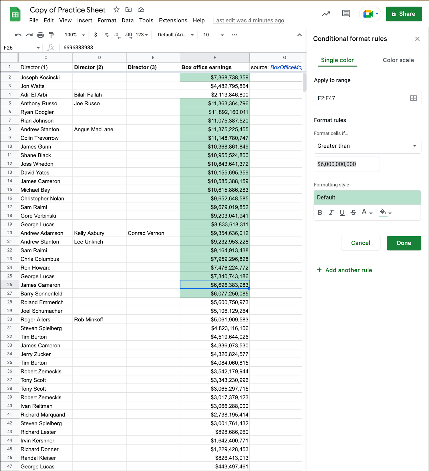
This will open the "Conditional format rules" panel on the right side of your screen. This panel is your control center for creating and managing all your formatting rules. It has three main parts:

• Apply to range: The cells your rule will affect.
• Format rules: The condition that a cell must meet (e.g., value is greater than, text contains).
• Formatting style: The visual change that will be applied (e.g., background color, bold text).

Highlighting Data with Single-Color Rules

The most common use of conditional formatting is to apply a single color to cells that meet a specific criterion. This is perfect for highlighting outliers, key values, or items that need attention.

The following video provides a clear walkthrough of how to set up a basic single-color rule based on a numerical value.

As you saw, the process is dynamic. If a cell's value changes and no longer meets the condition, the formatting is automatically removed. This is incredibly useful for trackers and live data.

Practical Exercise, Part 1: Highlight High-Value Invoices

Now, let's apply this to your My Freelance Invoices sheet.

1. Open your spreadsheet.
2. Select the entire range of your Amount (USD) column (e.g., D4:D100).
3. Open the Conditional formatting panel (Format > Conditional formatting).
4. Under "Format rules," select Greater than.
5. In the "Value or formula" box that appears, enter a value that represents a high-value project for you, for example, 500.
6. Under "Formatting style," choose a green background color.
7. Click Done.

Your high-value invoices should now be instantly visible with a green background.

Visualizing Data with a Color Scale

Sometimes, you don't just want to highlight specific values but visualize the entire spectrum of your data. A color scale is perfect for this. It applies a color gradient to your data range, for example, making the lowest values red, mid-range values yellow, and the highest values green. This gives you an immediate visual sense of the distribution of your numbers.

Let's return to the video to see how this works.

Practical Exercise, Part 2: Visualize Invoice Amounts

A color scale is a great way to get a feel for your income distribution.

1. With your Amount (USD) column still selected, click "Add another rule" in the conditional formatting panel.
2. This time, select the Color scale tab at the top of the panel.
3. You can choose a default color scheme. The "Green to yellow to red" or "White to green" options are good starting points.
4. Google Sheets will automatically set the lowest value in your range as the Minpoint and the highest as the Maxpoint.
5. Click Done.

You now have two rules on the same data. You'll see cells over $500 are still highlighted green (from the first rule), and all the cells have a faint color gradient applied from the second rule. In Google Sheets, if multiple rules apply to a cell, the rule that is listed first takes precedence. You can drag the rules in the panel to re-order them.

Expanding Your Rules: Text and Dates

Conditional formatting isn't limited to numbers. You can apply it to nearly any data type. For a freelance data researcher, two other rule types are particularly valuable:

• Text-based rules: Highlight cells where the text contains, starts with, or is exactly a certain word. This is great for flagging project types, client names, or a specific status like "Pending" or "Overdue."
• Date-based rules: Highlight dates that are before or after a certain day. This is essential for tracking deadlines. You can even use dynamic dates like today or in the past week.

Practical Exercise, Part 3: Flag Overdue Invoices

Let's add a critical rule to your invoice tracker.

1. Select your Due Date column.
2. Click "Add another rule".
3. Under "Format rules," select Date is before.
4. In the dropdown that appears, select today.
5. Under "Formatting style," choose a light red background to indicate urgency.
6. Click Done.

Any invoice with a due date in the past will now be automatically highlighted in red, ensuring you never lose track of late payments.

Conclusion

You have now equipped your invoice tracker with dynamic visual cues, a fundamental skill for efficient data analysis. Instead of manually searching for information, you've made the spreadsheet do the work for you, highlighting what's important at a glance.

Here are the main takeaways from today's lesson:

• Conditional formatting applies visual styles to cells based on "if-then" rules.
• Single-color rules are ideal for highlighting specific values, such as high numbers, specific text, or past-due dates.
• Color scales provide a visual gradient that helps you understand the distribution of numerical data.
• You can create rules based on numbers, text, dates, and more, making this a versatile tool for any dataset.

You can now highlight data, but what if you want to rearrange it? For example, you might want to see all your invoices listed from the highest amount to the lowest, or group them by client. In our next lesson, we will cover sorting, another essential technique for organizing your data for analysis.