Understanding Space Complexity

1. Total Space vs. Auxiliary Space

When we talk about space complexity, we need to be precise about what memory we are counting. This leads to two related but distinct concepts:

• Space Complexity (or Total Space): This is the total amount of memory used by an algorithm, including the space required to store the input data itself.
• Auxiliary Space: This is the extra or temporary memory that an algorithm uses during its execution, excluding the space taken by the inputs.

Auxiliary space is often the more interesting metric for comparing algorithms. Why? Because if you're sorting an array of n elements, any algorithm will have a total space complexity of at least O(n) just to hold the array. The real difference between algorithms lies in how much additional space they need to do their work.

As the article mentions, an algorithm's memory usage can be broken down into a few parts. For our purposes, the two most significant are:

1. Data Space: Memory used by variables, constants, and data structures.
2. Environment Stack: Memory used to manage function calls, which is especially important for recursive algorithms.

Let's see how to calculate these for some simple iterative algorithms.

2. Analyzing Space in Iterative Algorithms

Calculating space complexity often involves a line-by-line inspection of the code to identify where memory is allocated.

Let's consider a very simple function that sums two integers:

int sum(int a, int b) {
    int result = a + b;
    return result;
}

The inputs a and b take up a fixed amount of space. The local variable result also takes up a fixed amount of space. This memory usage doesn't change no matter how large the values of a and b are. Therefore, the auxiliary space is constant, or O(1).

Now, let's look at an algorithm that operates on an array.

This example is crucial. The total space grows linearly with the input size n because of the input array itself. However, the extra space needed (for the sum and the loop counter) remains constant. So, we say the function has O(n) total space complexity but O(1) auxiliary space complexity. This is characteristic of many in-place algorithms.

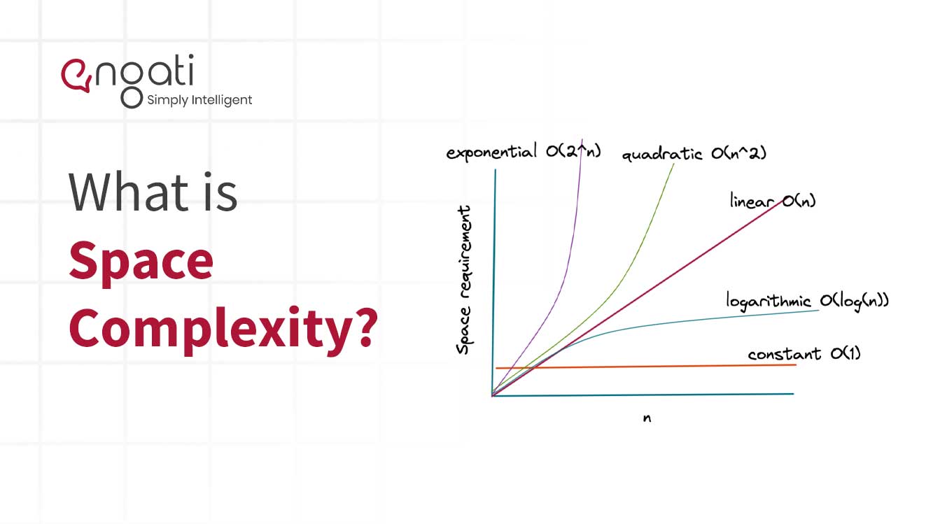
The following chart provides a helpful visual for how different complexity classes scale. An algorithm with O(1) space is highly efficient, while one with O(n) or higher will see its memory requirements grow with the input size.

3. The Space Complexity of Recursion

In the last lesson, we saw that recursive function calls have a time cost. They also have a space cost. Each time a function calls itself, the system must save its current state (local variables, parameters, return address) on the call stack. This saved state is called a stack frame.

If a function F(n) calls F(n-1), which calls F(n-2), and so on, a chain of stack frames builds up. The maximum number of frames on the stack at any one time determines the space complexity of the recursion.

This image visualizes how the call stack grows for a recursive Fibonacci function.

Let's analyze some of the recursive algorithms we've seen before, this time for their space complexity.

To summarize:

• Recursive Factorial: factorial(n) calls factorial(n-1) down to the base case, creating a call stack of depth n. The auxiliary space is O(n). This contrasts with the iterative version, which has O(1) auxiliary space.
• Quicksort: Its auxiliary space comes from the call stack. The depth depends on how balanced the partitions are, leading to O(log n) average-case space but O(n) worst-case space.
• Merge Sort: It requires O(log n) space for the call stack, but it also requires an O(n) auxiliary array to merge the sorted halves. The total auxiliary space is O(n) + O(log n), which simplifies to O(n).

4. The Space-Time Tradeoff

Often, you can make an algorithm faster by using more memory, or reduce its memory footprint at the cost of more computation time. This is known as the space-time tradeoff. Dynamic programming and memoization, which you'll study later, are prime examples of this principle.

By storing the results of fibonacci(k) in a memory table, we avoid recomputing the same values over and over. This is a classic example of trading increased space (O(n) for the table) for a massive reduction in time (from O(2^n) to O(n)).

Conclusion

In this lesson, you've learned how to analyze the second major dimension of an algorithm's performance: its space complexity.

Key Takeaways:

• Space Complexity measures an algorithm's memory usage relative to its input size.
• It's crucial to distinguish between Total Space (input + extra space) and Auxiliary Space (just the extra space). Auxiliary space is often more useful for comparing algorithms.
• Memory usage comes from variables and data structures (data space) and the function call stack (environment stack).
• Recursive algorithms consume space on the call stack proportional to the maximum depth of recursion.
• Algorithms often present a space-time tradeoff, allowing you to optimize for one resource at the expense of the other.

We have now covered the two main pillars of algorithmic resource analysis: time and space. With this foundation, our next lesson will move to a higher level of abstraction. We will explore how computer scientists classify the inherent difficulty of computational problems themselves into complexity classes like P, NP, and NP-complete.