P, NP, and NP-Complete: Understanding Computational Complexity

1. A Software Engineer's Dilemma

Imagine your boss gives you a challenging task: develop an algorithm for a new logistics application. The goal is to find the absolute most efficient route for a delivery truck to visit hundreds of cities. You spend weeks on it. Every fast algorithm you design fails to find the optimal route in some cases, and every algorithm that guarantees the optimal route is incredibly slow—so slow that it would take years to run for a large number of cities.

You don't want to report back that you've failed. What if the issue isn't your skill, but the nature of the problem itself?

This is precisely the value of understanding the complexity classes we'll discuss today. It allows you to distinguish between problems that are "tractable" (efficiently solvable) and those that are widely believed to be "intractable."

2. The Class P: Tractable Problems

The first and simplest class is P.

P stands for Polynomial time. It's the set of all decision problems that can be solved by an algorithm in a number of steps that is a polynomial function of the input size.

In simpler terms, if a problem has a known algorithm that runs in a time complexity like $O(n)$, $O(n\log n)$, $O(n^2)$, or any $O(n^k)$ for a constant $k$, that problem is in the class P.

These are the problems we consider "efficiently solvable" or tractable. Almost every algorithm you've studied so far—like sorting, binary search, and finding the shortest path in a graph with Dijkstra's algorithm—solves a problem in P.

3. The Class NP: Easy to Verify, Hard to Solve?

Next, we have the class NP. This is one of the most misunderstood terms in computer science.

A common misconception is that NP stands for "Non-Polynomial." This is incorrect. NP stands for Nondeterministic Polynomial time.

While the formal definition involves a theoretical "nondeterministic" computer that can magically guess correctly, a much more useful and intuitive definition is based on verification.

A problem is in NP if, given a proposed solution (called a "certificate" or "witness"), we can verify whether that solution is correct in polynomial time.

The Sudoku puzzle is a perfect analogy:

• Solving a large, blank Sudoku puzzle from scratch can be very difficult and time-consuming.
• Verifying a completed Sudoku grid to see if it follows all the rules is very fast and straightforward.

Because verifying a Sudoku solution is fast (polynomial time), the Sudoku problem is in NP.

The critical relationship between P and NP is that P is a subset of NP (P ⊆ NP). If a problem can be solved in polynomial time, its solution can certainly be verified in polynomial time (you can just ignore the proposed solution and solve it yourself to check).

This leads to the biggest unsolved question in computer science: Does P = NP?
If P = NP, it would mean that every problem for which a solution can be quickly verified can also be quickly solved. Most experts believe that P ≠ NP, meaning there are problems in NP that are not in P—they are easy to check but genuinely hard to solve.

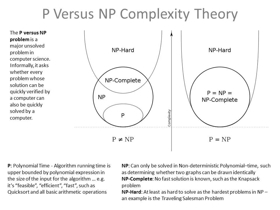
4. NP-Hard and NP-Complete: The Hardest of the Hard

Within the vast landscape of NP, two special categories define the "hardest" problems.

• NP-Hard: A problem is NP-Hard if it is at least as hard as any problem in NP. This means any problem in NP can be "reduced" (transformed) into an NP-Hard problem in polynomial time. An NP-Hard problem doesn't have to be in NP itself (e.g., optimization problems like finding the absolute best TSP tour, not just deciding if a tour of cost k exists).

• NP-Complete (NPC): A problem is NP-Complete if it meets two criteria:

  1. It is in NP (solutions can be verified in polynomial time).
  2. It is NP-Hard (every other problem in NP can be reduced to it).

NP-Complete problems are, in essence, the hardest problems in the class NP. The logistics problem from our intro—the Traveling Salesperson Problem (TSP)—is a classic example.

The concept of reduction is the linchpin. In 1971, the Cook-Levin theorem proved that the Boolean Satisfiability Problem (SAT) was NP-Complete. This was a monumental discovery because it gave us the first "hardest" problem. Since then, thousands of other problems have been proven to be NP-Complete by showing that SAT (or another known NPC problem) can be reduced to them.

This creates a chain reaction: if you could find a polynomial-time algorithm for any single NP-Complete problem, you would have effectively found one for all of them, proving that P = NP.

5. Practical Implications: What To Do About NP-Completeness

So, you've identified that your "iThingy" or logistics problem is NP-Complete. What now? This is where theory meets practice.

1. Stop searching for a perfect, efficient algorithm. The global community of top computer scientists hasn't found one in over 50 years. It's overwhelmingly likely that you won't either.
2. Change your goal. Instead of the optimal solution, aim for a good enough solution. This is where different strategies come into play.

To summarize the strategies for tackling an NP-Complete problem:

• Approximation: Design an algorithm that is guaranteed to find a solution within a certain percentage of the optimal one (e.g., a route that is no more than 10% longer than the absolute shortest).
• Heuristics: Use clever rules of thumb that often produce good solutions in practice but have no theoretical guarantee of optimality (e.g., a "greedy" approach for the TSP: "always go to the nearest unvisited city").
• Check Constraints: Is your input size always small? An exponential-time algorithm might be perfectly acceptable if n is never larger than 20.
• Look for Special Cases: Sometimes, a general NP-Complete problem becomes solvable in polynomial time if you add certain constraints. For example, the VERTEX-COVER problem is NP-complete on general graphs, but it's in P for bipartite graphs.

The practical impact is immense. Recognizing an NP-Complete problem saves you from wasting time on an impossible quest and redirects your efforts toward finding a practical, workable solution.

Conclusion

This lesson concludes our journey through the foundations of algorithmic analysis. We have moved from the nitty-gritty of counting operations and memory usage to the highest level of abstraction: classifying the intrinsic difficulty of problems themselves.

Key Takeaways:

• P: Problems solvable in polynomial time. These are considered "tractable."
• NP: Problems whose solutions can be verified in polynomial time. It is not known if P = NP.
• NP-Hard: Problems that are at least as hard as the hardest problems in NP.
• NP-Complete: The "hardest" problems within NP. A polynomial-time solution for one would mean P = NP.
• Practical Implication: Identifying a problem as NP-Complete is a crucial engineering insight. It tells you to shift your strategy from seeking a perfect, efficient solution to using approximations, heuristics, or solving for constrained special cases.

With this solid theoretical foundation, we are now ready to dive into the practical building blocks of efficient algorithms.

Preview of the Next Lesson:

In the next module, "Essential Data Structures Review," we will begin by revisiting the fundamental data structures—arrays, linked lists, stacks, and queues. We will analyze their performance characteristics, which are the tools you'll use to build the efficient algorithms for all the tractable problems you'll encounter.