Solving Recurrence Relations: Master Theorem & Recursion Trees

Hello! Welcome to the third lesson in our "Foundations of Algorithmic Analysis" module.

In our last two lessons, we built a solid understanding of how to describe an algorithm's efficiency using asymptotic notations like Big-O, Big-Omega, and Big-Theta. These tools are perfect for analyzing algorithms with simple loops. However, many powerful algorithms, especially those that follow a "divide and conquer" strategy, are written recursively. Analyzing them requires a different approach.

This lesson introduces recurrence relations, the mathematical language we use to describe the runtime of recursive algorithms. You will learn two powerful methods to solve these relations:

The Recursion Tree Method: An intuitive, visual approach that helps you understand what's happening "under the hood" of a recursive process.
The Master Theorem: A "cookbook" method that provides a quick and direct solution for a common class of recurrence relations.

By the end of this lesson, you'll be able to analyze the time complexity of many recursive algorithms you'll encounter throughout this course.

1. From Recursive Code to a Recurrence Relation

Before we can analyze a recursive algorithm, we need to describe its behavior mathematically. A recurrence relation breaks down the total time, T(n), into two parts:

The time spent in the recursive calls on smaller inputs.
The time spent on the non-recursive work within the function, like dividing the problem or combining the results.

Let's look at how recurrence relations are formed for some classic algorithms.

Time Complexity Analysis of Recursive Algorithms

The following article explains how to derive recurrence relations from the logic of a recursive algorithm. We'll focus on the general principle and a key example you'll see often: Merge Sort.

Please read the first two sections, up to and including the analysis of Merge Sort. Focus on how the structure of the mergeSort algorithm directly translates into its recurrence relation: T(n) = 2T(n/2) + cn.

As you saw, Merge Sort's recurrence T(n) = 2T(n/2) + cn tells us that the time to sort n elements is the time to sort two subproblems of size n/2, plus the linear-time cn work of merging the sorted halves.

Many divide-and-conquer algorithms have recurrences that fit the general form:
$T (n) = a T (n / b) + f (n)$
Where:

a is the number of subproblems.
n/b is the size of each subproblem.
f(n) is the cost of the work done outside the recursive calls.

Now, let's learn our first method for solving these equations.

2. The Recursion Tree Method: Visualizing the Work

The recursion tree method is a fantastic way to build intuition. We model the recursive calls as a tree, where each node represents the cost of a single subproblem. By summing the costs at each level of the tree, and then summing the totals for all levels, we can find the overall complexity.

Recursion tree method | Solving Recurrences | Data Structure & Algorithm | Gate Applied Course

This video provides an excellent walkthrough of how to build and analyze a recursion tree. It demonstrates the entire process, from expanding the initial recurrence to summing the costs to find the final complexity.

Watch the video from the beginning until 13:30. Pay close attention to these three key steps: Building the tree: How T(n) = 3T(n/4) + Cn^2 is expanded into levels of subproblems. Calculating cost per level: How the work done at each level is summed up. Summing the total cost: How the sum across all levels forms a geometric series, which simplifies to the final Big-O complexity.

The video you just watched used the recurrence T(n) = 3T(n/4) + cn^2. Here is a static image of that same process, which you can use as a reference.

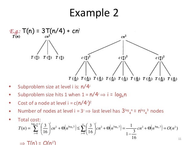
Recursion Tree Method Example — This diagram shows the step-by-step analysis of the recurrence `T(n) = 3T(n/4) + cn^2` using the recursion tree method. It illustrates the cost at each level (root, level 1, level 2, etc.) and culminates in a geometric series that is summed to find the total cost, which is `O(n^2)`.

The recursion tree method is powerful and works even for complex recurrences where subproblem sizes are unequal (e.g., T(n) = T(n/3) + T(2n/3) + n). However, it can be cumbersome. For a large class of common recurrences, there is a much faster way.

3. The Master Theorem: A "Cookbook" Solution

The Master Theorem provides a formula for solving recurrences of the form T(n) = aT(n/b) + f(n), where a ≥ 1, b > 1, and f(n) is an asymptotically positive function. It works by comparing the rate of work done at the root (f(n)) with the rate of work done at the leaves of the recursion tree.

The theorem is split into three cases, based on comparing f(n) to the term n^(log_b a). This critical value n^(log_b a) represents the asymptotic number of leaves in the recursion tree.

Let's see how these cases work in practice.

2.4.1 Masters Theorem in Algorithms for Dividing Function #1

The following video from Abdul Bari offers a very practical guide to applying the Master Theorem. He simplifies the comparison by looking at the exponent of n in f(n).

Please watch the video from the beginning to 16:51. It is broken down as follows: Introduction (0:00 - 1:18): Defines the parameters a, b, and the function f(n). It introduces the comparison between log_b(a) and k (where f(n) = Θ(n^k)). Case 1 (1:18 - 2:08 & 4:32 - 10:05): log_b(a) > k. The work at the leaves dominates. The video shows several examples. Case 2 (2:08 - 3:31 & 10:05 - 14:42): log_b(a) = k. The work is evenly distributed across levels. The video also covers important sub-cases involving logarithmic factors. Case 3 (3:31 - 4:32 & 14:42 - 16:51): log_b(a) < k. The work at the root dominates.

To summarize the Master Theorem, here is a concise reference for the three cases.

Lecture 20: Recursion Trees and the Master Method

This text provides a formal definition of the three cases of the Master Method (another name for the Master Theorem) and gives a clear example for each one.

Read the section titled 'The Master Method' and the three examples that follow. Note how it compares f(n) directly to n^(log_b a), which is equivalent to comparing k and log_b a.

4. A Worked Example: Merge Sort

Let's solidify our understanding by analyzing the Merge Sort recurrence, T(n) = 2T(n/2) + O(n), using both methods.

Using the Recursion Tree Method:

Level 0 (Root): We do cn work.
Level 1: We have 2 subproblems of size n/2. Each does c(n/2) work. Total work: 2 * c(n/2) = cn.
Level 2: We have 4 subproblems of size n/4. Each does c(n/4) work. Total work: 4 * c(n/4) = cn.
...and so on.
Tree Depth: The problem size is halved at each level, so the depth of the tree is log₂(n).
Total Work: We do cn work at each of the log₂(n) levels. The total time is the sum of the work at all levels, which is cn * log₂(n), or Θ(n log n).

Using the Master Theorem:

The recurrence is T(n) = 2T(n/2) + O(n).
a = 2 (number of subproblems)
b = 2 (input size is halved)
f(n) = O(n) = O(n^1), so k = 1.
Now, we calculate the critical value: log_b(a) = log₂(2) = 1.
We compare log_b(a) with k. Here, 1 = 1. This falls into Case 2.
The result for Case 2 is Θ(n^k log n) = Θ(n^1 log n) = Θ(n log n).

Both methods give us the same, correct answer. The Master Theorem is much faster once you're familiar with it, but the recursion tree helps you understand why the answer is what it is.

Conclusion

In this lesson, you've added two indispensable tools to your analytical toolkit for handling recursive algorithms.

Key Takeaways:

Recurrence relations are mathematical equations that model the time complexity of recursive algorithms. The common form is T(n) = aT(n/b) + f(n).
The Recursion Tree Method provides a visual and intuitive way to solve recurrences by summing the work done at each level of recursion. It is highly versatile.
The Master Theorem is a "shortcut" for solving recurrences that fit the aT(n/b) + f(n) form. It involves comparing f(n) to n^(log_b a) and applying one of three cases.

In our next lesson, we will shift our focus from time to another critical resource: memory. We will learn how to analyze the space complexity of an algorithm, completing our foundational understanding of algorithmic analysis.

Recommended resources