Dynamic Programming vs. Greedy vs. Divide & Conquer

1. The Defining Properties: A Refresher

The key to distinguishing these paradigms lies in two properties we've discussed before: Optimal Substructure and Overlapping Subproblems.

• Optimal Substructure: An optimal solution to the problem contains within it optimal solutions to its subproblems. All three paradigms (D&C, Greedy, and DP) rely on this property.
• Overlapping Subproblems: A recursive algorithm solves the same subproblems over and over again. This is the crucial property that separates DP from D&C.

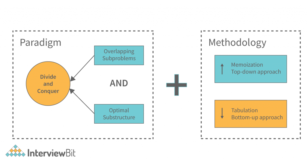
Let's quickly review this distinction.

To summarize:

• Divide and Conquer: Uses optimal substructure but subproblems are independent (e.g., sorting the left half of an array has no effect on sorting the right half).
• Dynamic Programming: Uses optimal substructure and subproblems are overlapping (e.g., calculating fib(5) and fib(4) both require fib(3)).

This handles the D&C vs. DP distinction. The more challenging distinction is often between Greedy and DP.

2. Greedy vs. Dynamic Programming

Both Greedy and DP are typically used for optimization problems and both require optimal substructure. The key difference is how they make choices.

• A Greedy algorithm makes one choice—the one that looks best at the moment—and sticks with it. It never reconsiders.
• A DP algorithm explores all possible choices and picks the best one. It finds the global optimum by solving all relevant subproblems.

This video offers a great initial comparison.

The fundamental question that separates Greedy from DP is this: Does the problem have the Greedy Choice Property?

The Greedy Choice Property means that a globally optimal solution can be arrived at by making a sequence of locally optimal choices. If you can prove this property holds, you can use a fast and efficient greedy algorithm. If you can find a counterexample where a locally optimal choice prevents you from reaching the global optimum, you must use Dynamic Programming.

3. Case Study: The Interval Scheduling Problem

Let's see this in action with a classic problem that perfectly illustrates the boundary between Greedy and DP. We'll explore two variations of the Interval Scheduling problem. The following resource is a lecture from MIT OpenCourseWare that walks through this beautifully.

Part A: Unweighted Interval Scheduling (A Greedy Solution)

First, consider the basic problem: given a set of intervals, find the maximum number of mutually compatible (non-overlapping) intervals.

Here, a greedy strategy works. We'll see that by always picking the interval that finishes earliest, we are guaranteed to find an optimal solution.

The key takeaway is that for the unweighted version, the greedy choice is "safe." Picking the interval that finishes first leaves the maximum possible time for other intervals to be scheduled, ensuring we don't prematurely block off better future choices.

Part B: Weighted Interval Scheduling (A DP Solution)

Now, let's change the problem slightly: each interval i has a weight w_i. The goal is to find a set of compatible intervals with the maximum total weight.

This small change breaks the greedy strategy. The interval that finishes earliest might have a tiny weight, and by picking it, we might prevent ourselves from picking a much heavier interval that starts later. We are now forced to make a more complex decision for each interval: either we take it, or we don't. This signals the need for DP.

The DP formulation for the weighted problem looks like this: for each interval i, we consider two possibilities:

1. Include interval i: The total weight is w_i + the optimal solution for the subproblem of intervals that are compatible with i.
2. Exclude interval i: The total weight is the optimal solution for the subproblem of all intervals except i.

The optimal solution is the maximum of these choices, considered for all intervals. This exploration of choices is the hallmark of DP.

4. A Decision Framework

We can summarize our discussion into a mental flowchart for approaching a new optimization problem:

1. Check for Optimal Substructure. Can the problem be broken down into smaller, similar subproblems whose optimal solutions contribute to the main solution?

   • If No, none of these paradigms apply directly.
   • If Yes, proceed to the next question.

2. Try to formulate a Greedy choice. Can you identify a simple, locally optimal rule for making a choice?

   • If Yes, try to prove it's correct or, more practically, try hard to find a counterexample.
   • If you find a counterexample -> You likely need Dynamic Programming.
   • If you are confident the greedy choice is always safe -> Use a Greedy algorithm.

3. If you need DP (or D&C), check for subproblem dependency. When you break the problem down recursively, are the subproblems independent?

   • If Yes (independent subproblems) -> Use Divide and Conquer.
   • If No (overlapping subproblems) -> Use Dynamic Programming.

This table provides a final, concise summary of the key differences.

Conclusion

You've now reached a significant point in your study of algorithms. Recognizing the underlying structure of a problem is a more abstract and powerful skill than simply memorizing algorithms.

Key Takeaways:

• Divide and Conquer is for problems with optimal substructure and independent subproblems.
• Greedy algorithms are for optimization problems with optimal substructure and the Greedy Choice Property. They are fast but require proof of correctness. The best way to challenge a greedy idea is to look for a counterexample.
• Dynamic Programming is for optimization problems with optimal substructure and overlapping subproblems. It is more powerful than a greedy approach because it exhaustively explores all choices to guarantee a global optimum.
• The transition from unweighted to weighted interval scheduling is the canonical example of a problem crossing the boundary from Greedy to DP.

Preview of the Next Lesson:
We are now moving to the final topic of our course: Backtracking. While DP is an intelligent way to solve optimization problems, backtracking is a methodical way to explore all possible configurations to find a solution that satisfies a set of constraints (e.g., solving a Sudoku puzzle). It can be seen as an organized, intelligent form of brute-force search, and it provides a powerful tool for a different class of problems.