Backtracking: Depth-First Search in State-Space Trees

1. The Core Idea: Searching for Solutions

At its heart, backtracking is a systematic way of trying out all possible sequences of decisions to find a solution. Unlike a greedy algorithm that commits to a choice, backtracking is prepared to undo a choice and try another if the current path isn't leading to a valid solution.

This approach is particularly useful for problems like solving Sudoku, navigating a maze, or finding all permutations of a set of items. The key is that we build a solution step-by-step, and at each step, we check if we've violated any of the problem's constraints.

Let's begin with a video that introduces this general method.

This idea of exploring "all possible solutions" can be visualized as a tree structure, which is central to understanding how backtracking works.

2. The State-Space Tree

The set of all possible paths or decision sequences in a backtracking problem can be organized into a state-space tree.

• The root of the tree represents the initial state, before any decisions have been made.
• Each node in the tree represents a partial solution or a specific state reached after a sequence of choices.
• Each branch represents a choice that moves us from one state to another.
• The leaves of the tree represent either complete, valid solutions or dead ends.

Imagine you're solving a maze. The root is the entrance. Each time you reach an intersection, you create branches in the tree for each possible turn (left, right, straight). A path from the root to a leaf represents a complete journey through the maze.

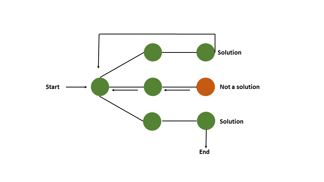
To formalize this, let's look at how the problem's solution space is modeled as this tree.

A node is promising if the partial solution it represents can still lead to a valid complete solution. It's non-promising if we can determine that no matter what further choices we make from this point, we can never reach a valid solution. This is where the "intelligence" of backtracking comes in—we stop exploring as soon as a node becomes non-promising.

3. Traversing the Tree: A Depth-First Approach

Now for the central part of our learning outcome: how does backtracking actually explore this state-space tree? It does so using a Depth-First Search (DFS).

Recall from our graph traversal module that DFS explores as far as possible along each branch before backtracking. This is exactly what a backtracking algorithm does:

1. Start at the root.
2. Choose one branch and go down one level.
3. Repeat this process, going deeper and deeper into the tree.
4. If you reach a valid solution, record it.
5. If you reach a non-promising node (a dead end) or a leaf that isn't a solution, you backtrack: you go back up to the parent node and try the next unexplored branch.

This video makes the connection between backtracking and DFS explicit.

With your software engineering background, you'll appreciate a more formal definition. The following resource presents backtracking search as a recursive algorithm and analyzes its complexity, which aligns with the DFS traversal pattern.

The memory complexity of $O(D)$ is a direct result of the DFS approach. Since we only need to store the current path from the root to the node we are visiting, the memory usage is proportional to the depth of the tree, not its total number of nodes. This makes backtracking feasible for very large search spaces where a BFS approach (which would require storing all nodes at a given level) would run out of memory.

4. The Power of Pruning

If backtracking just explored every single node in the state-space tree, it would be a simple brute-force search. Its true power lies in pruning: the ability to discard large portions of the state-space tree.

As soon as we determine a node is "non-promising" because it violates a problem constraint, we don't just stop at that node—we refuse to generate any of its descendants. This is the "backtracking" step in action. By cutting off entire subtrees, we can achieve massive performance gains over a naive exhaustive search.

This concept is also known as applying a bounding function.

Conclusion

In this lesson, we have laid the conceptual foundation for the backtracking paradigm. It's a powerful technique for solving problems that can be modeled as a search for a valid configuration among many possibilities.

Key Takeaways:

• Backtracking is an algorithmic paradigm for solving constraint satisfaction problems by systematically exploring all possible candidates.
• The search space is conceptualized as a state-space tree, where paths from the root represent partial solutions.
• Backtracking explores this tree using a Depth-First Search (DFS) traversal, which makes it very memory-efficient ($O(D)$ space).
• Its efficiency comes from pruning: it abandons a path as soon as it determines the path cannot lead to a valid solution (i.e., the node becomes "non-promising").

Preview of the Next Lesson:

Now that we understand the theory, it's time to put it into practice. In the next lesson, we will apply backtracking to solve the classic N-Queens problem. We'll define the state, identify the constraints that allow for pruning, and walk through the construction of a recursive solution.