Tree Dynamic Programming Fundamentals

Introduction

This lesson focuses on a special, but very common, type of DAG: the tree. Since a tree is inherently acyclic, all the principles of DP on DAGs apply, but the structure of a tree allows for an even more intuitive recursive approach.

Our goal is to learn how to approach DP problems on trees. We will do this by dissecting a classic problem: finding the maximum path sum in a binary tree. You will learn to define the appropriate DP state for a tree node and structure a recursive solution that correctly gathers information from subproblems. This directly continues our deep dive into DP, applying it to a new and important data structure.

1. From DAGs to Trees: A Natural Progression

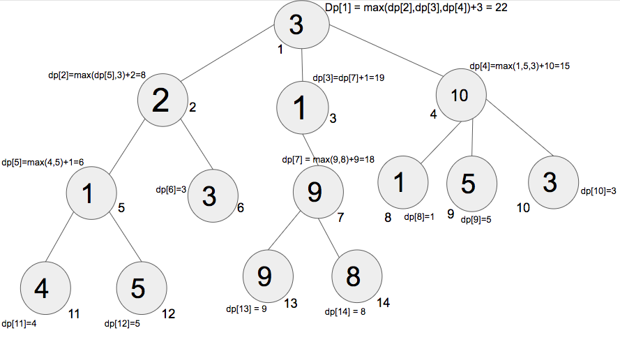
In the last lesson, the key was to find a linear ordering of vertices (a topological sort) so we could solve subproblems in the correct sequence. For a tree, this ordering is naturally provided by its structure. If we root a tree, a post-order traversal (visiting left child, right child, then the root) is effectively a topological sort. It ensures we have computed the answers for all of a node's children before we compute the answer for the node itself.

This leads to a powerful and elegant pattern for DP on trees:

• The subproblems are defined on the subtrees.
• The state for a node u, let's call it dp[u], represents the solution for the subtree rooted at u.
• We write a recursive function (typically a Depth-First Search) that computes dp[u] based on the results from its children, dp[child1], dp[child2], etc.

The following resource explains this concept clearly.

Sometimes, the state dp[u] needs to store more than one piece of information. For example, in the "Weighted Maximum Independent Set" problem discussed in the same resource (resource_id=[LINK](https://cgi.cse.unsw.edu.au/~cs4128/19t3/lectures/5-dp.pdf), section starting on page 28), the state for a node u needs to track two values: the max weight including u and the max weight excluding u. This is a common pattern in tree DP problems.

2. Case Study: Binary Tree Maximum Path Sum

Let's apply this thinking to a concrete problem. The "Binary Tree Maximum Path Sum" is a LeetCode Hard problem, but it breaks down elegantly with a DP approach.

The Problem: Given a binary tree with integer values (which can be positive or negative), find the maximum sum of any non-empty path. A path can start and end at any node and does not need to pass through the root. Critically, a path can only "bend" or "turn" at one node.

First, let's get a solid grasp of the problem's definition and the core intuition behind the solution.

As the reading highlights, the crux of the problem lies in the recursive function for a node u. This function must do two things:

1. Calculate and return the maximum path sum starting at u and going downwards into one of its subtrees (left or right). This is the value u can contribute to its parent. A path can't go up to a parent and then down both of the parent's other branches.
2. Calculate and update a global maximum with the path sum where u is the "peak" or "highest point". This path consists of u.value plus the downward paths from its left and right children. This value is a candidate for the final answer but is not returned to the parent.

This distinction is the most important concept in solving this problem.

3. The Algorithm and a Visual Walkthrough

Let's formalize the algorithm based on the insights from the previous section. We'll use a recursive DFS approach.

Algorithm:

1. Initialize a global variable max_so_far to negative infinity. This will store the answer.
2. Define a recursive helper function, say dfs(node).
3. Base Case: If node is null, it contributes nothing to a path. Return 0.
4. Recursive Step:
   a. Recursively call dfs on the left and right children. Let the results be left_gain and right_gain.
   b. Crucially, ignore negative gains. A path would rather not extend into a subtree that provides a negative sum. So, we compute left_gain = max(0, dfs(node.left)) and right_gain = max(0, dfs(node.right)).
5. Update Global Maximum: Calculate the maximum path sum with the current node as the peak: current_max_path = node.val + left_gain + right_gain. Update max_so_far = max(max_so_far, current_max_path).
6. Return Value: The function must return the maximum gain it can provide upwards to its parent. This path can only go down one side. So, return node.val + max(left_gain, right_gain).
7. The final answer is the value in max_so_far after the initial call dfs(root).

Now, let's watch a video that walks through this exact logic on an example.

4. Complexity Analysis and Common Pitfalls

Given your interest in the "why," let's briefly analyze the performance and potential mistakes.

• Time Complexity: $O(N)$, where $N$ is the number of nodes in the tree. The recursive DFS visits each node exactly once.
• Space Complexity: $O(H)$, where $H$ is the height of the tree. This space is used by the recursion call stack. In the worst case of a skewed tree, this can be $O(N)$. For a balanced tree, it's $O(\log N)$.

The resource from AlgoMonster that you read earlier also has an excellent section on common pitfalls. The two most important ones to remember are:

1. Forgetting to handle negative contributions: Not using max(0, ...) on the recursive results is a common bug.
2. Returning the wrong value: The recursive function must return the "upward-contributing" path (node.val + max(left_gain, right_gain)), not the "peak" path (node.val + left_gain + right_gain).

Conclusion

In this lesson, we specialized our knowledge of DP on DAGs to the more structured case of trees. We saw that a post-order traversal provides a natural order for solving subproblems, leading to elegant recursive solutions.

Key Takeaways:

• DP on trees is typically implemented with a recursive DFS function that works its way up from the leaves.
• The core challenge is defining the DP state. For each node, you must clearly distinguish between the information needed to solve the problem at that node versus the information it must pass up to its parent.
• In the Maximum Path Sum problem, this meant distinguishing between the "peak" path (a candidate for the global answer) and the "straight" path (the value returned from the recursion).
• Handling edge cases, like negative path contributions, is critical for correctness.

Preview of the Next Lesson:
So far, we've explored several powerful algorithmic paradigms: Divide and Conquer, Greedy algorithms, and now various forms of Dynamic Programming. But when you face a new problem, how do you decide which strategy to use? In our next lesson, we will focus on exactly that: developing the intuition to distinguish when a problem calls for DP versus a greedy or divide and conquer approach.