Implementing Linear Regression with NumPy: Prediction and Cost Functions

1. From Math to Code: The Power of Vectorization

To implement these formulas efficiently, we won't loop through each data point one by one. Instead, we'll use NumPy to perform the calculations on the entire dataset at once. This technique is called vectorization, and it's a cornerstone of high-performance scientific computing and machine learning.

Let's reconsider our hypothesis function for an entire dataset. If we have $m$ data points, we can represent our single feature as a vector $x$ and our model's predictions as a vector $\hat{y}$.

The equation $h_{\theta }(x^{(i)})={\theta }_0+{\theta }_1{x}^{(i)}$ for every data point $i$ can be expressed using linear algebra. We can combine our parameters into a vector $\theta$:

And we can augment our feature matrix $X$ by adding a column of ones. This "dummy" feature corresponds to the intercept parameter ${\theta }_0$. If our original features are in a column vector, our new $X$ matrix looks like this:

With this setup, the predictions for all $m$ data points can be calculated in a single matrix-vector multiplication:

This single operation is far more efficient than a for loop.

To see this concept explained with a focus on the implementation, let's look at an article that builds a linear regression model from scratch.

2. Implementing the Prediction Function

Now, let's turn the vectorized formula $\hat{y}=X\cdot \theta$ into a Python function. Using NumPy, this becomes incredibly straightforward. We will define a function that takes the feature matrix X and the parameter vector theta as inputs and returns the predictions.

The following article presents a clean, function-based implementation.

As you saw, the implementation is just a single line, harnessing the power of NumPy's dot method for matrix multiplication. Here is what it looks like:

import numpy as np

def predict(X, theta):
  """
  Calculates the predictions of a linear regression model.

  Args:
    X (np.ndarray): The feature matrix (with a column of ones for the bias).
                    Shape: (m, n+1), where m is samples, n is features.
    theta (np.ndarray): The model parameters (weights and bias).
                        Shape: (n+1, 1).

  Returns:
    np.ndarray: The predicted values. Shape: (m, 1).
  """
  return X.dot(theta)

This predict function is our hypothesis $h_{\theta }(X)$ in code.

3. Implementing the Cost Function

With our prediction function ready, we can now implement the MSE cost function, $J(\theta )$. Recall the formula:
$J(\theta )=\frac{1}{2m}\sum (\hat{y}-y{)}^2$

Let's break down the implementation using NumPy:

1. Calculate predictions ($\hat{y}$): We'll call the predict(X, theta) function we just wrote.
2. Calculate the errors: This is a simple element-wise subtraction: predictions - y.
3. Square the errors: We can use the ** 2 operator, which NumPy applies to each element in the array.
4. Sum the squared errors: np.sum() will sum all the elements in the resulting array.
5. Average and scale: Multiply the sum by 1 / (2 * m), where m is the number of samples.

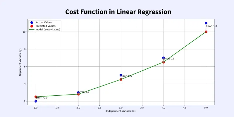
The image below visually represents the errors we are calculating—the vertical distances between the actual data points and the model's prediction line. Our cost function will aggregate all these errors into one number.

Now, let's look at a code implementation of this function.

The video provides a great, concise implementation. For our purposes, we will wrap this logic in a dedicated function, similar to how we handled the prediction. The Dev.to article provides a perfect example of this.

Here is the complete cost function, with comments explaining each part:

def cost(X, y, theta):
  """
  Calculates the Mean Squared Error cost for linear regression.

  Args:
    X (np.ndarray): Feature matrix. Shape: (m, n+1).
    y (np.ndarray): Actual target values. Shape: (m, 1).
    theta (np.ndarray): Model parameters. Shape: (n+1, 1).

  Returns:
    float: The MSE cost.
  """
  m = len(y) # Number of training examples
  predictions = predict(X, theta)
  squared_errors = (predictions - y) ** 2
  



  # The formula is 1/(2*m) * sum_of_squared_errors
  return (1 / (2 * m)) * np.sum(squared_errors)

4. Putting It All Together: A Concrete Example

We've defined the two functions. Let's see them in action with a small, concrete example. This will make the abstract code tangible.

Let's imagine we have 4 data points:

• x values: 1, 2, 3, 4
• y values: 2, 4, 5, 4

And let's start with an initial guess for our parameters: ${\theta }_0=0$ and ${\theta }_1=1$. This corresponds to the line $y=x$. What is the cost for this initial guess?

# 1. Prepare the data
# Our feature values (x)
x_values = np.array([[1], [2], [3], [4]]) 



# Our target values (y)
y_values = np.array([[2], [4], [5], [4]]) 



# Get the number of samples
m = len(y_values)




# 2. Add the bias term (a column of ones) to X
X_b = np.c_[np.ones((m, 1)), x_values] # np.c_ is a handy way to concatenate columns




# 3. Initialize parameters (theta)
# Let's start with a guess: theta0 = 0, theta1 = 1
theta_guess = np.array([[0], [1]])




# 4. Use our functions
# Get the predictions for our guess
predictions_guess = predict(X_b, theta_guess)
print(f"Our initial predictions:\n{predictions_guess}\n")




# Calculate the cost for our guess
cost_value = cost(X_b, y_values, theta_guess)
print(f"The cost for our initial guess (theta0=0, theta1=1) is: {cost_value}")

Running this code would produce:

Our initial predictions:
[[1.]
 [2.]
 [3.]
 [4.]]

The cost for our initial guess (theta0=0, theta1=1) is: 1.25

This cost of 1.25 gives us a concrete measure of how "wrong" our initial line $y=x$ is for this dataset. If we chose different values for theta_guess, we would get a different cost.

Conclusion

In this lesson, you have successfully translated the core mathematical equations of linear regression into functional Python code. You have taken a significant step from abstract theory towards concrete implementation.

Key Takeaways:

• Vectorization is the practice of using matrix operations to perform calculations on entire datasets at once, and it is key to writing efficient ML code.
• The prediction function $h_{\theta }(X)$ can be implemented as a simple matrix multiplication X.dot(theta), provided the feature matrix X includes a bias column of ones.
• The MSE cost function $J(\theta )$ is implemented by using the prediction function, calculating the squared errors, and finding their scaled average using NumPy operations like np.sum().
• You now have two essential building blocks: a function to make predictions and a function to evaluate how good those predictions are.

Preview of the Next Lesson:
We can now calculate the cost for any given set of parameters $\theta$. But how do we find the $\theta$ that gives the lowest possible cost? Doing it by manual trial and error is not feasible.

In the next lesson, we will implement gradient descent, the optimization algorithm that automatically and intelligently finds the optimal values for $\theta$. We will use the very functions you built today inside the gradient descent loop to iteratively minimize the cost and "train" our model.