Mean Squared Error: The Cost Function

1. The Need for a "Cost" Metric

Imagine you have a scatter plot of data points. You can draw an infinite number of straight lines through that data. Our goal is to find the single line that best represents the underlying trend. To do this objectively, we need a way to score each potential line—a metric that tells us how "wrong" it is. This score is what we call the cost or loss.

A lower cost means a better fit. The line with the lowest possible cost is our "best-fit line."

Let's begin by reading a short article that introduces this core idea and sets the stage for building our own cost function.

2. Deriving the Cost Function from First Principles

Now, let's derive this cost function step-by-step. Our goal is to create a single number that represents the total error of our model across all data points.

Step 1: The Error for a Single Data Point

For any single data point, the error is simply the difference between the value our model predicts and the actual value. This vertical distance is often called the residual.

• Actual value: $y^{(i)}$
• Predicted value: $h_{\theta }(x^{(i)})$
• Error (residual): ${\text{error}}^{(i)}=h_{\theta }(x^{(i)})-y^{(i)}$

Our first instinct might be to sum up these errors for all $m$ points in our training set. However, there's a problem with this approach.

Step 2: The Flaw in Summing Raw Errors

What happens if our model predicts a value that is too high for one point (a positive error) and a value that is too low for another (a negative error)? If we simply add them, they might cancel each other out, giving us a deceptively small total error.

To understand this problem and see how we can fix it, let's continue with the article from Built In.

As the article explains, taking the absolute value of the error (leading to Mean Absolute Error or MAE) is a valid solution. However, another, more common approach in regression is to square the error.

Step 3: Squaring the Error

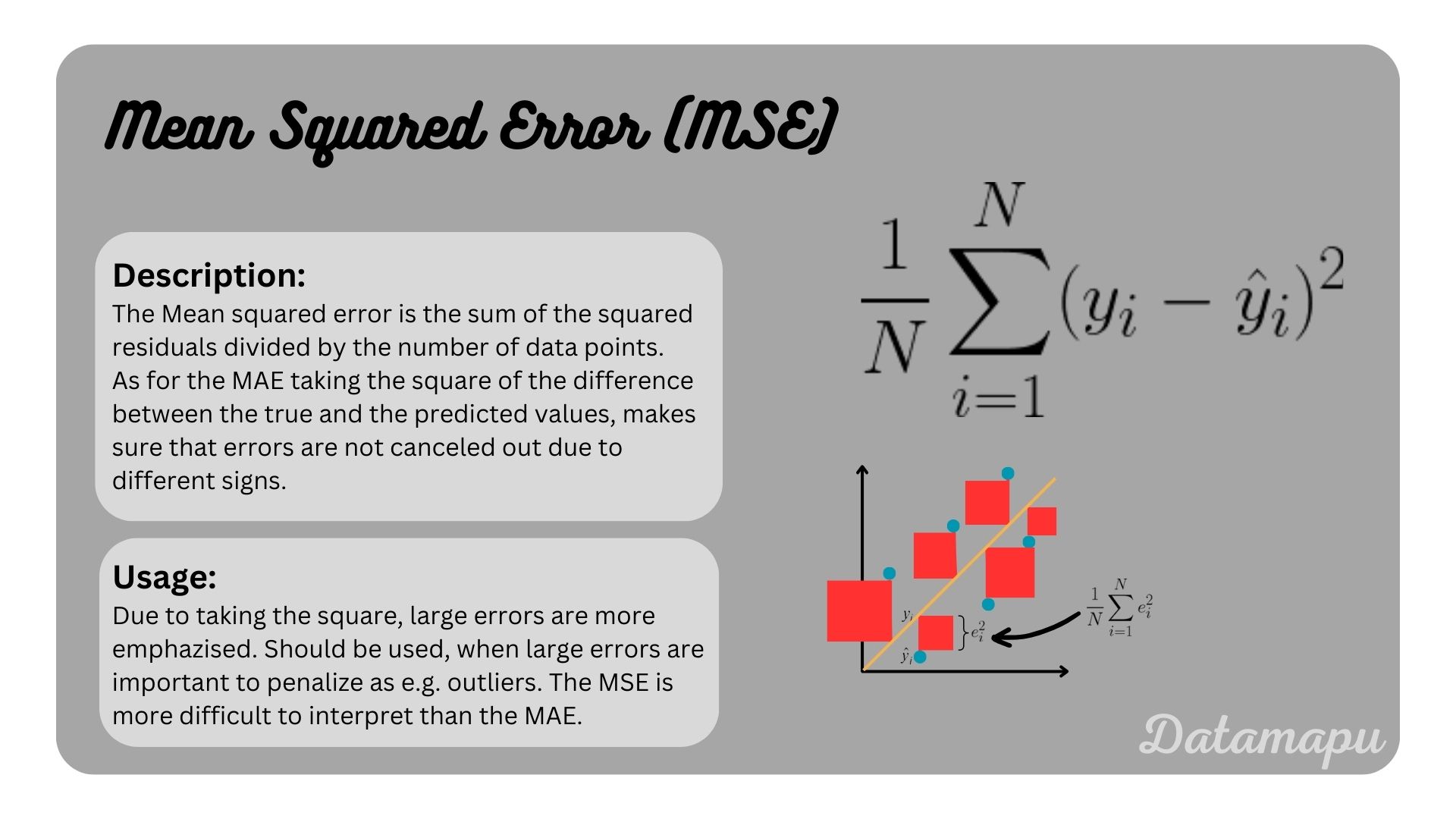
Instead of taking the absolute value, we can square the difference: $(h_{\theta }(x^{(i)})-y^{(i)}{)}^2$. This also solves the cancellation problem by ensuring every error term is positive. Squaring the error has two desirable properties:

1. It penalizes larger errors more heavily. An error of 2 becomes 4, but an error of 10 becomes 100. This means the model will be strongly motivated to fix its biggest mistakes.
2. It creates a smooth, differentiable function. The squared function has a clean derivative, which is extremely useful for optimization algorithms like gradient descent, a topic we will cover soon. This is a significant advantage over the absolute value function.

The image below shows this concept visually. The error for each point is the vertical line, and the cost associated with that point is the area of the red square.

Step 4: Averaging the Squared Errors

Finally, to get a single cost value for the entire dataset, we sum up all the individual squared errors and divide by the number of data points, $m$. This gives us the Mean Squared Error (MSE).

3. The Formal Definition of the MSE Cost Function

Now that we've built the intuition, let's formalize the MSE cost function, which we denote as $J(\theta )$.

To see this presented in a lecture format, let's turn to a classic explanation from Andrew Ng's course at Stanford.

As explained in the video, the formal equation for the cost function $J(\theta )$ is:

Let's break this down one last time:

• $\theta$: These are the parameters of our model (e.g., ${\theta }_0$ and ${\theta }_1$). The cost $J$ is a function of these parameters. Our goal is to find the values of $\theta$ that minimize $J$.
• $m$: The number of examples in our training set.
• ${\sum }_{i=1}^m$: A sum over all the training examples, from the first ($i=1$) to the last ($i=m$).
• $h_{\theta }(x^{(i)})$: The prediction of our model for the $i$-th data point. Remember, this is our hypothesis function, e.g., ${\theta }_0+{\theta }_1{x}^{(i)}$.
• $y^{(i)}$: The true, actual value for the $i$-th data point.
• $(h_{\theta }(x^{(i)})-y^{(i)}{)}^2$: The squared error for a single data point.
• $\frac{1}{m}$: This makes it the mean squared error. It ensures the cost isn't dependent on the size of the dataset.
• $\frac{1}{2}$: This is a constant included for mathematical convenience. When we later compute the derivative of this function to minimize it, this $\frac{1}{2}$ will conveniently cancel out the exponent '2' from the squared term, simplifying our calculations. It doesn't change the final values of $\theta$ that we find.

For a final, text-based summary of this derivation, please review the following resource.

4. A Concrete Example

Abstract formulas are best understood with a concrete example. The image below walks through the calculation of the MSE cost for a very simple model and a small dataset.

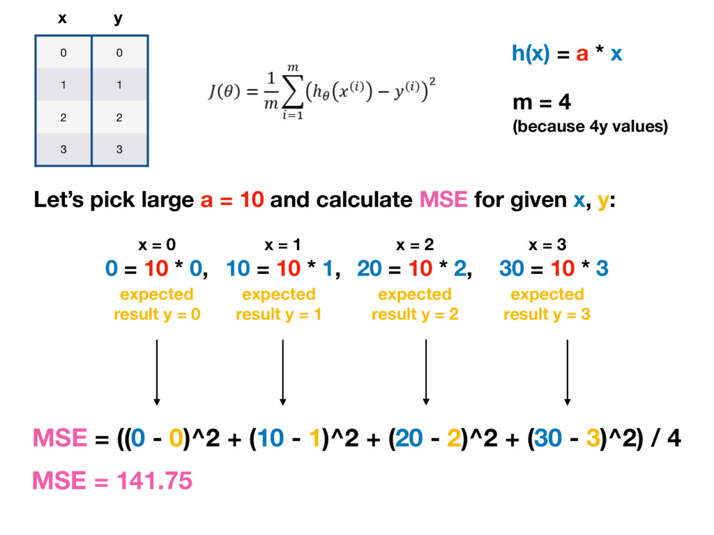
Following the steps in the image, we see that for a specific choice of parameters (in this case, a line with slope 10 and intercept 0), the cost is 141.75. If we were to choose a different slope, say a=8, we could repeat the calculation and get a different cost. The goal of training is to find the value of a that results in the lowest possible cost.

5. Visualizing the Cost Function

This leads to a powerful insight: the cost $J$ is itself a function of our model's parameters $\theta$. For a simple linear regression with one feature, our parameters are ${\theta }_0$ (intercept) and ${\theta }_1$ (slope). This means the cost function is a 3D surface, where the x- and y-axes are ${\theta }_0$ and ${\theta }_1$, and the z-axis is the cost $J({\theta }_0,{\theta }_1)$. Our goal is to find the point (${\theta }_0,{\theta }_1$) at the very bottom of this surface.

Let's watch a clip that visualizes a simpler, 2D version of this, showing how the cost changes as we vary just one parameter.

Conclusion

In this lesson, we have moved from the abstract need for a "best-fit line" to a concrete, mathematical tool for finding it. We have derived, from first principles, the Mean Squared Error (MSE) cost function.

Key Takeaways:

• A cost function quantifies a model's total error into a single number, allowing us to objectively compare different models.
• For linear regression, the standard cost function is Mean Squared Error (MSE), which is the average of the squared differences between predicted and actual values.
• The formula is $J(\theta )=\frac{1}{2m}{\sum }_{i=1}^m(h_{\theta }(x^{(i)})-y^{(i)}{)}^2$.
• We use MSE because it penalizes large errors heavily and its mathematical properties (being smooth and differentiable) make it easy to minimize.
• The goal of training a linear regression model is to find the set of parameters ($\theta$) that results in the minimum possible cost.

Preview of the Next Lesson:
We now have a precise definition of our model ($h_{\theta }(x)$) and a way to measure its error ($J(\theta )$). The next logical step is to bring these theoretical concepts into the practical realm of code.

In the next lesson, we will begin our transition from theory to application by addressing the outcome: Implement the prediction and cost functions for linear regression using NumPy. You will write Python code that directly translates these mathematical formulas, setting the stage for the subsequent lesson where we will build an algorithm to automatically find the parameters that minimize this cost.