Understanding Linear Regression: Concepts and Assumptions

Introduction

Welcome to our first lesson in the "Supervised Learning: Regression Models" module. In the previous module, we established a robust framework for evaluating machine learning models, culminating in our exploration of k-fold cross-validation. You now understand how to measure a model's performance and ensure that your evaluation is reliable.

Now, we shift our focus from evaluating models to building them. We'll start with one of the most fundamental and interpretable algorithms in machine learning. This lesson addresses the learning outcome: Explain the concept of linear regression and its underlying assumptions.

We will explore the core idea of modeling relationships with a straight line and, crucially, discuss the "rules of the game"—the assumptions that must be true for the model to produce trustworthy results. Understanding these foundations is a critical step toward the strategic, first-principles thinking required to build powerful AI systems.

1. The Concept of Linear Regression

At its heart, regression analysis is about understanding and modeling the relationship between variables. We have a set of input variables, called features (or independent variables), and a target variable we want to predict, called the label (or dependent variable). The goal is to learn a function that maps the features to the label.

Linear regression is a specific type of regression analysis where we assume this relationship can be modeled by a straight line.

Core Idea: Finding the "Best-Fit Line"

Imagine you have data on house sizes and their corresponding prices. You'd intuitively expect that, on average, larger houses are more expensive. If you were to plot this data, you could try to draw a single straight line that best summarizes this trend. This is the essence of linear regression.

This "best-fit line" serves two purposes:

Interpretation: It tells us how the variables are related. The steepness of the line, for example, tells us how much the price tends to increase for each additional square foot.
Prediction: Once we have the line, we can use it to predict the price of a new house that wasn't in our original dataset, just by knowing its size.

Linear Regression Visual with Equation and Error — This image shows the fundamental concept of linear regression. The blue dots are our data points (e.g., houses of different sizes and prices). The red line is the "best-fit line" that the model learns. The equation defines this line, and the term ε (epsilon) represents the error—the vertical distance from each data point to the line.

To formalize this, let's watch a short segment from a Stanford lecture that introduces the core problem and the key terminology.

Stanford CS229: Machine Learning - Linear Regression and Gradient Descent | Lecture 2 (Autumn 2018)

Let's begin with a foundational explanation from Andrew Ng's machine learning course at Stanford. He uses the classic housing price example to define the problem that linear regression solves and introduces the formal terminology we'll be using.

Watch the first 4 minutes (00:00 to 03:58). Focus on understanding these key terms: Supervised Learning: Why this task is considered 'supervised'. Regression Problem: What makes this a regression task as opposed to a classification one. Training Set: The data we use to learn. Hypothesis: The function, h(x), that our algorithm outputs to make predictions.

2. The Model's Equation: The Hypothesis Function

As the video explained, the output of our learning algorithm is a hypothesis function, which we denote as $h (x)$ . In linear regression, this function is simply the equation of a line.

Simple Linear Regression (One Feature)

For a problem with a single input feature $x$ (e.g., house size) and a target label $y$ (e.g., price), the equation is:

h (x) = β_{0} + β_{1} x

$β_{0}$ (beta-zero) is the intercept: the predicted value of $y$ when $x$ is 0. It's where the line crosses the y-axis.
$β_{1}$ (beta-one) is the coefficient or slope: it represents the change in $y$ for a one-unit increase in $x$ .
$β_{0}$ and $β_{1}$ are the model's parameters (often denoted as $θ_{0}$ and $θ_{1}$ in machine learning literature). The goal of "training" the model is to find the best possible values for these parameters.

Multiple Linear Regression (Multiple Features)

Most real-world problems are more complex. A house's price doesn't just depend on its size; it also depends on the number of bedrooms, the age of the house, its location, etc. When we use more than one feature, it's called multiple linear regression.

The equation simply extends to include the additional features:

h (x) = β_{0} + β_{1} x_{1} + β_{2} x_{2} + \dots + β_{n} x_{n}

$x_{1}, x_{2}, \dots, x_{n}$ are the different features (e.g., $x_{1}$ = size, $x_{2}$ = number of bedrooms).
$β_{1}, β_{2}, \dots, β_{n}$ are the coefficients for each feature, representing the influence of that feature on the final prediction.
$β_{0}$ is still the intercept.

The next video clip shows how this generalization is formally represented.

Stanford CS229: Machine Learning - Linear Regression and Gradient Descent | Lecture 2 (Autumn 2018)

Now, let's generalize this concept from a single feature to multiple features. This part of the lecture explains how the hypothesis function expands and introduces the standard notation used in machine learning, which you'll see throughout your AI studies.

Watch from 04:39 to 08:20. Pay attention to how the equation changes to include multiple features (x_1, x_2, etc.) and their corresponding parameters ( heta_1, heta_2, etc.). Note the convention of setting x_0=1 to handle the intercept term ( heta_0) elegantly.

3. The Underlying Assumptions

A linear regression algorithm will always produce a line, but that line is only meaningful and reliable if certain conditions—or assumptions—are met. Understanding these assumptions is what separates a novice from an expert. It allows you to diagnose when a model is likely to fail and why.

First, let's get a quick overview of the key assumptions.

Assumptions of Linear Regression

Before we dive into each assumption, let's get a high-level summary. This article from GeeksforGeeks provides a concise list of the key assumptions a linear regression model relies on.

Read only the section titled 'Assumptions of the Linear Regression'. This will serve as a quick reference for the concepts we're about to explore in more detail.

Now, let's explore the most critical of these assumptions with more intuitive, visual explanations. The following image provides a great visual summary that we will refer to.

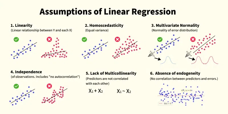
Assumptions of Linear Regression — This image visually summarizes the core assumptions of linear regression. For each one, it contrasts a scenario where the assumption holds (✅) with one where it is violated (❌). We will now unpack the most important of these.

Assumption 1: Linearity

This is the most fundamental assumption. It states that the relationship between the features and the label is, in fact, linear. If you're trying to model a curved relationship with a straight line, your model will be inherently flawed.

Regression assumptions explained!

Let's explore the linearity assumption. The following video provides an excellent intuitive explanation of what it means and, more importantly, how you can spot if it's being violated.

Watch from 04:41 to 09:25. Focus on the example of lung function vs. age. Understand what an 'incorrect functional form' means and how looking at a 'residual plot' (a plot of the errors) can help you diagnose this problem.

Assumption 2: Homoscedasticity (Constant Error Variance)

This is a technical term for a simple idea: the model's errors should be consistent across the entire range of predictions. A violation, called heteroscedasticity, occurs when the errors get larger or smaller as the feature values change. For example, your model might be very accurate for low-priced houses but highly inaccurate for expensive ones. This is a problem because it means the model's reliability is not uniform.

Regression assumptions explained!

Next is Homoscedasticity, which means 'constant error variance'. This assumption is about the consistency of the model's errors.

Watch from 14:06 to 17:35. Pay close attention to the income vs. expenditure example. Note how the spread of the data points 'fans out' as income increases, and how this pattern appears in the residual plot. This violation is called heteroscedasticity.

Assumption 3: Independence of Errors (No Autocorrelation)

This assumption states that the errors for each data point are independent of one another. A violation, called autocorrelation, is most common in data collected over time (time-series data). For example, with stock market data, a large prediction error today might be followed by another large error tomorrow. This suggests there's a pattern in the errors that the model isn't capturing.

Regression assumptions explained!

The third assumption concerns the independence of errors. This is especially relevant when your data has a natural order, like a time sequence.

Watch from 19:05 to 22:50. Understand why this is primarily a concern for time-series data and how a violation, known as autocorrelation, often looks like a 'snaking' pattern in the residual plot.

Assumption 4: No Multicollinearity

This assumption applies to multiple linear regression. It means that the input features should not be highly correlated with each other. For instance, if you include both the size of a house in square feet and its size in square meters as features, they are perfectly correlated. This creates a redundancy that confuses the model; it can't determine how much of the price change is due to one feature versus the other.

Regression assumptions explained!

When we have multiple input features, we need to worry about Multicollinearity. This assumption states that our input features should be independent of each other.

Watch from 30:19 to 35:20. Focus on the example of motor accidents vs. number of cars and residents. The key idea is that if two input variables are highly related, the model struggles to 'isolate the individual effects' of each one.

Conclusion

In this lesson, we have laid the theoretical groundwork for linear regression, one of the foundational building blocks of machine learning.

Key Takeaways:

Linear regression models the relationship between features (inputs) and a continuous label (output) by fitting a straight line (or a hyperplane in multiple dimensions).
The model is represented by a hypothesis function $h (x)$ , which is a linear equation whose parameters (coefficients) are learned from data.
For the model's results and interpretations to be reliable, several key assumptions must be met:
- Linearity: The underlying relationship is linear.
- Homoscedasticity: The variance of errors is constant.
- Independence of Errors: Errors are not correlated with each other (no autocorrelation).
- No Multicollinearity: Input features are not highly correlated with each other.

Preview of the Next Lesson:
We've defined the model and the rules it must follow. But a crucial question remains: how do we find the best straight line? What does "best" even mean? To answer this, we need a way to measure how well a given line fits the data.

In the next lesson, we will explore this by focusing on the next learning outcome: Derive the cost function (Mean Squared Error) for linear regression. This function will give us a precise mathematical way to quantify our model's error, paving the way to learn how to minimize it.

Recommended resources

Introduction

1. The Concept of Linear Regression

2. The Model's Equation: The Hypothesis Function

Simple Linear Regression (One Feature)

Multiple Linear Regression (Multiple Features)

3. The Underlying Assumptions

Assumption 1: Linearity

Assumption 2: Homoscedasticity (Constant Error Variance)

Assumption 3: Independence of Errors (No Autocorrelation)

Assumption 4: No Multicollinearity

Conclusion