Introduction
Welcome back! In our last lesson, you successfully built two of the most critical components of a linear regression model: the predict function to make predictions and the cost function to measure how wrong those predictions are. We ended with a key question: how do we find the model parameters (theta, or w and b) that give the lowest possible cost?
Today, we answer that question by implementing Gradient Descent, the optimization algorithm that will train our model. This algorithm is the engine that drives the learning process in many machine learning models. By the end of this lesson, you will have a complete, working linear regression model trained from scratch.
Our learning outcome is to implement gradient descent to train a simple linear regression model from scratch. We will:
- Understand the intuition behind gradient descent.
- Calculate the gradients (derivatives) of our cost function.
- Implement the iterative update rule to minimize the cost and find our optimal parameters.
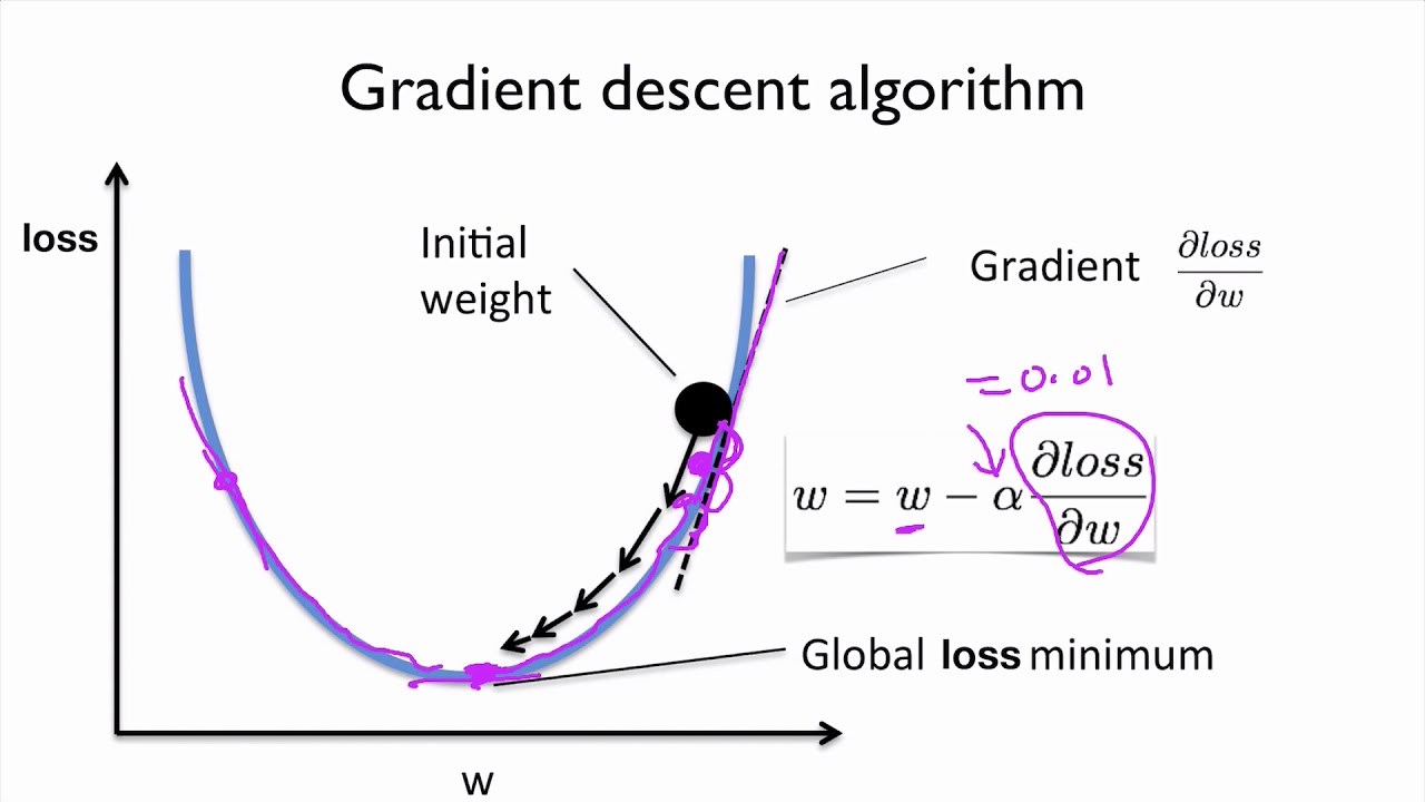
Let's start with the core concept. Imagine our cost function as a landscape with hills and valleys. Our goal is to find the absolute lowest point in this landscape. Gradient descent is an algorithm for doing just that: starting somewhere on a hill and taking steps downhill until we reach the bottom.
1. The Intuition of Gradient Descent
Before we dive into the math and code, it's essential to build a solid intuition for how gradient descent works. It’s an iterative process:
- Start with an initial, random guess for the model parameters (e.g., slope
w=0, interceptb=0). - Calculate the direction of steepest ascent at your current position. In calculus, this direction is given by the derivative (or gradient).
- Step in the opposite direction (downhill) by a small amount. This new position corresponds to a new set of parameters with a slightly lower cost.
- Repeat steps 2 and 3 until the step size becomes negligible, meaning you've arrived at the bottom of the valley.
The following video from StatQuest provides an excellent, step-by-step walkthrough of this process. It first simplifies the problem by optimizing only the intercept, which makes the core idea very clear.
Gradient Descent, Step-by-Step
Watch this segment from 'Gradient Descent, Step-by-Step' to build a strong intuition for the algorithm's mechanics.
Watch the video from 01:56 to 05:38, which explains the process of finding the optimal intercept by plotting the loss function and visualizing the 'downhill' steps. Then, watch from 09:41 to 13:30, which details how each step is calculated using the derivative and a 'learning rate', and how the steps get smaller as we approach the minimum.
Two key concepts from the video are:
- The Derivative (Slope): The steepness of the cost function at our current point tells us how big a step to take. A steep slope means we're far from the minimum, so we take a big step. A shallow slope means we're close, so we take a small step.
- The Learning Rate: This is a small number that controls the size of each step we take. It prevents us from overshooting the minimum.
2. The Mathematics: Finding the Direction
To implement gradient descent, we need to mathematically compute the "direction of steepest descent." This is done by calculating the gradient of the cost function. The gradient is a vector of partial derivatives, with one partial derivative for each parameter in our model.
In our last lesson, our cost function was:
Where the prediction . For consistency with most resources and to simplify the derivative, we'll use the Mean Squared Error (MSE), which drops the factor:
Our task is to find the partial derivatives of with respect to w (the weight or slope) and b (the bias or intercept).
The following resource provides a clear, step-by-step derivation of these partial derivatives. Since you prefer a theory-first approach, working through this derivation is a valuable exercise.
Gradient Descent - Machine Learning Visualized
The article 'Gradient Descent - Machine Learning Visualized' provides a concise and clear mathematical derivation of the gradients for a linear regression model.
First, read the section 'Loss Function: Mean Squared Error' to re-familiarize yourself with the cost function formula. Then, carefully study the sections 'Loss Function in Terms of W' and 'Loss Function in Terms of b'. Follow the chain rule application to understand how the final gradient formulas are derived.
After applying the chain rule, we arrive at these two crucial formulas for the gradients:
The partial derivative with respect to w:
The partial derivative with respect to b:
These formulas tell us exactly how to calculate the slope of the cost function for w and b at any given point. We now have our "downhill" direction.
3. Implementing the Gradient Descent Algorithm
Now we can combine the intuition and the math to write the code. The core of gradient descent is the update rule, where we adjust our parameters in the opposite direction of the gradient. We repeat this update for a fixed number of iterations (epochs).
The update rules for w and b are:
Here, (alpha) is the learning rate.
Let's implement this. We will create a gradient_descent function that takes the current parameters and data, computes the gradients, and returns the updated parameters. The article from datahacker.rs provides an excellent, clean implementation of this logic.
#002 Machine Learning - Linear Regression Models
This article, '#002 Machine Learning - Linear Regression Models', shows a complete Python implementation. We will focus on the code that performs the gradient descent step.
Read section '4. Implementing A Linear Regression Model In Python (From Scratch)'. Focus on the fit() method within the LinearRegression class. Observe how it implements the gradient descent loop: it calculates y_pred, then calculates the derivatives D_w and D_b, and finally updates the parameters self.w and self.b using the learning rate lr.
Now, let's write our own gradient_descent function from scratch, building upon the predict and cost functions from our previous lesson. Notice how the gradient formulas are implemented efficiently using NumPy's vectorized operations.
import numpy as np


# Let's assume the functions from the previous lesson are available
# We will use 'w' and 'b' for slope and intercept for clarity

def predict(X, w, b):
  """
  Calculates predictions for a simple linear regression model.
  X is a vector of features (m, 1).
  """
  return X * w + b

def cost(X, y, w, b):
  """
  Calculates the Mean Squared Error cost.
  """
  m = len(y)
  predictions = predict(X, w, b)
  squared_errors = (predictions - y) ** 2
  return (1 / m) * np.sum(squared_errors)

def gradient_descent(X, y, w, b, learning_rate, epochs):
  """
  Trains a linear regression model using gradient descent.

  Args:
    X (np.ndarray): Feature values. Shape (m, 1).
    y (np.ndarray): Target values. Shape (m, 1).
    w (float): Initial weight/slope.
    b (float): Initial bias/intercept.
    learning_rate (float): Step size for each iteration.
    epochs (int): Number of iterations to run.

  Returns:
    tuple: The final optimized weight (w) and bias (b).
  """
  m = float(len(y))
  cost_history = []

  for i in range(epochs):


    # 1. Get current predictions
    y_pred = predict(X, w, b)


    # 2. Calculate the gradients based on the formulas
    D_w = (-2/m) * np.sum(X * (y - y_pred))
    D_b = (-2/m) * np.sum(y - y_pred)


    # 3. Update the parameters
    w = w - learning_rate * D_w
    b = b - learning_rate * D_b


    # Optionally, track the cost to see if it's decreasing
    if i % 100 == 0:
        current_cost = cost(X, y, w, b)
        cost_history.append(current_cost)
        print(f"Epoch {i}: Cost {current_cost}")

  return w, b, cost_history
4. Training the Model: A Full Example
We have all the pieces. Let's use our gradient_descent function to train a model on some sample data and find the best-fit line.
# --- 1. Generate some sample data ---
np.random.seed(42) # for reproducibility
X_train = 2 * np.random.rand(100, 1)
y_train = 4 + 3 * X_train + np.random.randn(100, 1) # Line is y = 3x + 4 + noise


# --- 2. Set hyperparameters ---
learning_rate = 0.01
epochs = 1000


# --- 3. Initialize parameters ---
w_initial = 0.0
b_initial = 0.0


# --- 4. Train the model ---
print("Starting training...")
w_final, b_final, cost_history = gradient_descent(X_train, y_train, w_initial, b_initial, learning_rate, epochs)
print("Training complete.")


# --- 5. See the results ---
print(f"\nFinal parameters:")
print(f"w (slope): {w_final}")
print(f"b (intercept): {b_final}")


# The true values were w=3 and b=4. Our results should be close!
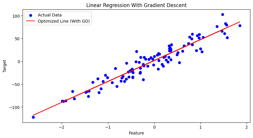
If you run this code, you'll see the cost decreasing every 100 epochs, and the final w and b will be very close to the true values of 3 and 4 that we used to generate the data.
To visualize our result, we can plot the original data along with the line created by our final, optimized parameters.
Conclusion
Congratulations! You have just implemented and trained a machine learning model from the ground up. You've gone from the core theory of linear regression to a practical, working implementation of gradient descent.
Key Takeaways:
- Gradient Descent is an iterative optimization algorithm that minimizes a cost function by repeatedly stepping in the direction opposite to the gradient.
- The gradient is a vector of partial derivatives, and , which points in the direction of the steepest ascent of the cost function.
- The update rule (
parameter := parameter - learning_rate * gradient) is the core mechanism of learning in this model. - The entire process involves initializing parameters, and then looping for a number of epochs to compute gradients and update the parameters, thereby progressively reducing the cost.
Preview of the Next Lesson:
Building models from scratch is the best way to understand their inner workings, which is fundamental to your polymath goal. However, for practical applications, we rarely re-implement these algorithms. Instead, we use highly-optimized, well-tested libraries.
In the next lesson, "Fit and interpret a linear regression model using scikit-learn," you will see how to accomplish everything we did today in just a few lines of code using Python's premier machine learning library, scikit-learn. This will be the first step in leveraging powerful tools to build complex AI systems more efficiently.