Linear Regression with scikit-learn

The Scikit-learn Workflow

Think of scikit-learn as a toolkit of pre-built, highly-optimized machine learning components. While we used gradient descent, scikit-learn's LinearRegression model uses a direct mathematical solution called Ordinary Least Squares (OLS) for fitting, which is much faster for this specific type of model. For more complex models, it uses advanced versions of gradient descent internally.

The beauty of scikit-learn is its consistent API. The process for training most supervised learning models follows the same four steps.

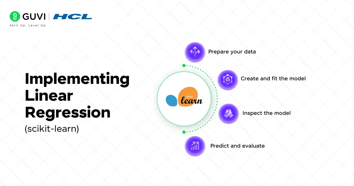
Here's how these steps relate to what we've already built:

1. Prepare Data: We separate our data into features (X) and the target variable (y). This is identical to how we prepared X_train and y_train for our own functions.
2. Create & Fit Model:
   • model = LinearRegression(): This is like creating a blueprint for our model, ready to learn the parameters.
   • model.fit(X, y): This single command executes the entire training process. It's the equivalent of our gradient_descent function running its loop to find the optimal slope and intercept.
3. Inspect Model: After fitting, we can check the learned parameters. The model stores them as model.coef_ (our w) and model.intercept_ (our b).
4. Predict & Evaluate:
   • model.predict(X_new): This works just like our own predict function, using the learned parameters to estimate outcomes for new data.

Fitting Your First Model with Scikit-learn

Let's walk through this process with a simple, practical example: predicting house prices based on their area. The following video provides an excellent demonstration. We will focus on the core steps of fitting the model and making a prediction.

Let's review the key lines of code from the video, which encapsulate the entire process:

import pandas as pd
from sklearn.linear_model import LinearRegression
import matplotlib.pyplot as plt




# 1. Prepare Data
df = pd.read_csv('homeprices.csv')
X = df[['area']] # Features (needs to be a 2D array or DataFrame)
y = df['price']  # Target




# 2. Create and Fit Model
model = LinearRegression() # Create the model object
model.fit(X, y)           # Train the model (find the best w and b)




# 3. Make a Prediction
area_to_predict = [[3300]] # New data must also be 2D
predicted_price = model.predict(area_to_predict)

print(f"Predicted price for a 3300 sq. ft. home: ${predicted_price[0]:.2f}")

Notice how clean and concise this is. The complexity of the gradient descent loop is completely handled by the .fit() method.

Interpreting the Learned Model

Fitting a model is only half the task. A crucial part of machine learning, especially in its application to real-world problems, is understanding what the model has learned. What is the relationship between house area and price according to our model?

The answer lies in the model's learned parameters: the intercept and the coefficient(s). In scikit-learn, these are stored in the model object after fitting.

• model.intercept_: This is a scalar value representing the b in our equation $y=wx+b$. It's the predicted value of y when x is 0.
• model.coef_: This is a NumPy array containing the coefficient for each feature. For simple linear regression, it will have one value: our w or slope.

Let's formalize this.

As the article explains, the interpretation is as follows:

• Intercept: The predicted price of a house with 0 square feet. In this context, it might not have a practical meaning but is a necessary component for positioning the regression line correctly.
• Coefficient: For every one-unit increase in the feature (i.e., for every additional square foot of area), the model predicts the price will increase by the value of the coefficient.

Let's retrieve these values from the model we just discussed.

# Assuming 'model' is the fitted LinearRegression object from before




# Get the learned parameters
intercept = model.intercept_
slope = model.coef_[0] # coef_ is an array, so we take the first element

print(f"Intercept (b): {intercept:.2f}")
print(f"Coefficient/Slope (w): {slope:.2f}")




# Manually verify the prediction for 3300 sq. ft.
manual_prediction = slope * 3300 + intercept
print(f"Manual prediction: ${manual_prediction:.2f}")
print(f"Model prediction:  ${predicted_price[0]:.2f}")

This confirms that model.predict() is simply applying the equation $y=wx+b$ using the parameters it found during the .fit() process.

From Simple to Multiple Linear Regression

Our from-scratch model handled one feature (X). Real-world problems often involve many features. For example, a house price is affected by area, number of bedrooms, age, location, etc. This is called multiple linear regression.

The scikit-learn workflow remains almost exactly the same. The only difference is that X is now a matrix with multiple columns, and model.coef_ will be an array with one coefficient for each feature.

This next video demonstrates how to build a model using the Boston housing dataset, which includes multiple features. It also introduces the important concept of splitting your data into training and testing sets, which we'll cover formally in a later module.

The interpretation for multiple regression coefficients is:

"Holding all other features constant, a one-unit increase in this feature is associated with a change of [coefficient value] in the target variable."

This ability to handle multiple features with no change in workflow is a key reason why libraries like scikit-learn are so powerful.

Conclusion

In this lesson, you have bridged the gap between theoretical understanding and practical application. You've seen how the concepts of fitting and predicting, which you built from scratch, are abstracted into simple, powerful commands in scikit-learn.

Key Takeaways:

• Scikit-learn abstracts complexity: It provides a high-level API (.fit(), .predict()) that handles the underlying optimization, allowing you to focus on the modeling problem itself.
• Fitting is training: The .fit(X, y) method is where the model learns the optimal parameters from the data.
• Interpretation is key: The learned parameters are stored in the intercept_ and coef_ attributes.
• intercept_ (b) is the baseline prediction when all features are zero.
• coef_ (w) represents the change in the predicted target for a one-unit change in a feature, holding all other features constant.
• The workflow is consistent for both simple (one feature) and multiple (many features) linear regression.

Preview of the Next Lesson:
Our linear regression model assumes a straight-line relationship between features and the target. But what if the relationship is curved? In our next lesson, we will learn about Polynomial Regression. You will discover how we can extend the linear regression framework to capture these non-linear patterns, making our models even more flexible and powerful.