Polynomial Regression for Non-Linear Data

When a Straight Line Isn't Enough

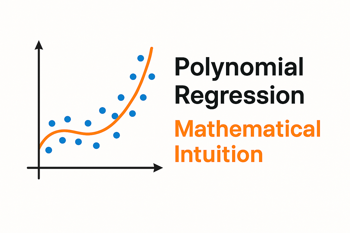
Imagine plotting data where the underlying pattern is a curve. If we try to fit a standard linear regression model, it will draw the best possible straight line, but it will fail to capture the essence of the relationship.

This failure of a simple model to capture the underlying trend is called underfitting. To fix this, we need a model that can bend. This is where polynomial regression comes in.

The Theory: Bending the Line with Polynomials

To understand polynomial regression, let's first recall the equation for a simple linear model:
$y={\beta }_0+{\beta }_{1}x+ϵ$
Here, $y$ is the target, $x$ is the feature, ${\beta }_0$ is the intercept, ${\beta }_1$ is the slope, and $ϵ$ is the error term.

Polynomial regression extends this equation by adding higher-order powers of the feature $x$. A second-degree (or quadratic) polynomial regression model looks like this:
$y={\beta }_0+{\beta }_{1}x+{\beta }_2{x}^2+ϵ$
By adding the $x^2$ term, we give the model the ability to create a parabolic curve. We can add even higher powers to create more complex curves. The general form of a polynomial regression model of degree $h$ is:
$Y={\beta }_0+{\beta }_{1}X+{\beta }_2{X}^2+\dots +{\beta }_h{X}^h+ϵ$

To solidify this foundational theory, please read the following brief introduction.

The key insight from the reading is that even though the model describes a non-linear relationship between $Y$ and $X$, it is linear in its coefficients (${\beta }_0,{\beta }_1,{\beta }_2,\dots$). The algorithm's job is to find the best values for these coefficients, and from the algorithm's perspective, this is a linear problem.

The following video provides an excellent walkthrough of these core concepts with visual examples.

The "Trick": Feature Engineering

So, if we're using a linear regression algorithm to fit a non-linear curve, how does that work? The answer lies in a powerful technique called feature engineering.

Instead of changing the algorithm, we change the data we feed into it.

Consider the quadratic equation: $y={\beta }_0+{\beta }_{1}x+{\beta }_2{x}^2$.
Let's create a new feature, let's call it $x_2$, where $x_2=x^2$. If we substitute this into our equation, we get:
$y={\beta }_0+{\beta }_{1}x+{\beta }_2{x}_2$
This is the exact form of a multiple linear regression model, which you saw in the previous lesson! The model doesn't know or care that $x_2$ is just the square of $x$. It treats them as two independent features and finds the best coefficients (${\beta }_1$ and ${\beta }_2$) for them.

By transforming our single feature x into multiple features (x, x^2, x^3, etc.), we can use a linear regression model to fit a complex curve.

This next video explains this transformation process beautifully.

This idea of "changing the data, not the model" is a fundamental concept in machine learning. It's a prime example of the kind of thinking that allows you to solve complex problems with simpler, well-understood tools.

The Danger: Choosing the Right Degree

If adding an $x^2$ term is good, is adding up to $x^{20}$ even better? Not necessarily. This brings us to one of the most important concepts in all of machine learning: the bias-variance tradeoff, which manifests here as a choice between underfitting and overfitting.

• Underfitting (High Bias): If the degree of our polynomial is too low (e.g., using a straight line for curved data), the model is too simple. It can't capture the underlying pattern.
• Overfitting (High Variance): If the degree is too high, the model becomes too flexible. It will start to wiggle and contort itself to pass through as many data points as possible, essentially "memorizing" the noise in the training data. This model will look great on the data it was trained on, but it will fail miserably when asked to make predictions on new, unseen data because it hasn't learned the true underlying relationship.

The goal is to find the "sweet spot"—a model that is complex enough to capture the true pattern but not so complex that it mistakes noise for a signal.

The video from Kody Simpson also has an excellent segment illustrating this trade-off.

Determining the optimal degree is a key part of the modeling process. In practice, this is often done by evaluating model performance on a separate test set for different degrees and choosing the one that generalizes best.

Conclusion

In this lesson, you have moved beyond straight lines and learned how to model the curves that are common in real-world data. You've discovered that you can achieve this without abandoning the linear regression framework you're familiar with, but by cleverly engineering your features.

Key Takeaways:

• Polynomial regression models non-linear relationships by adding higher-order terms ($x^2,x^3,\dots$) of a feature to the regression equation.
• It is still considered a linear model because the equation is linear in its coefficients (${\beta }_i$).
• The core mechanism is feature engineering: transforming the original feature set into a new, higher-dimensional one that a linear algorithm can use to fit a curve.
• Choosing the polynomial degree involves a crucial trade-off. A low degree can lead to underfitting, while a high degree can lead to overfitting.

Preview of the Next Lesson:
We've talked about "good" and "bad" fits, but how do we measure this numerically? In the next lesson, you will learn about key evaluation metrics for regression, such as Mean Squared Error (MSE) and R-squared. These metrics will allow you to quantitatively compare different models and make data-driven decisions about which one is best.