Clustering Performance Evaluation with Silhouette Score

Introduction

In our last lesson, you successfully implemented the k-means algorithm and learned how to use the Elbow Method and the Silhouette Score to select an optimal number of clusters, $k$ . We treated the silhouette score as a guide for choosing a hyperparameter.

Today, we will elevate its role from a selection tool to a powerful diagnostic metric. The learning outcome for this lesson is to evaluate clustering performance using metrics like the silhouette score. You will learn to go beyond the single average score and interpret detailed silhouette plots to assess the quality, shape, and separation of your clusters, and even identify potentially misclassified data points. This deeper understanding of evaluation is crucial for building robust and meaningful unsupervised learning models.

What Makes a "Good" Cluster?

Before we can evaluate clustering, we must define what we're looking for. Intuitively, a good clustering result has two key properties:

Cohesion: The data points within a single cluster should be close to each other. We can think of this as intra-cluster tightness.
Separation: Different clusters should be far apart from each other. We can think of this as inter-cluster distance.

An ideal clustering algorithm creates groups that are internally dense and well-separated from other groups. The silhouette score is a metric designed to measure exactly this balance.

To build on your theoretical understanding, let's watch a short video that clearly explains these two concepts and how they form the basis of the silhouette coefficient.

Silhouette Score for clustering Explained | Silhouette (clustering)- Validating Clustering Models

The video 'Silhouette Score for clustering Explained' by Unfold Data Science provides a very clear, plain-language explanation of cohesion and separation and how they are measured.

Watch the video from the beginning until 05:59. Focus on: How the video defines 'cohesion' and 'separation'. The calculation of the variable 'a', which measures cohesion. The calculation of the variable 'b', which measures separation.

Deconstructing the Silhouette Score

As the video explained, the silhouette score for a single data point $i$ is calculated using two values:

$a_{i}$ : Cohesion. The average distance from point $i$ to all other points in its own cluster. A small value for $a_{i}$ is desirable, as it means the point is close to its cluster-mates.
$b_{i}$ : Separation. The average distance from point $i$ to all points in the nearest neighboring cluster. A large value for $b_{i}$ is desirable, meaning the next closest cluster is far away.

Understanding the Silhouette Score Components — This diagram illustrates the two components of the silhouette score for a point `i`. `a(i)` measures the average distance within its own cluster (cohesion), while `b(i)` measures the distance to the nearest neighboring cluster (separation).

These two values are then combined into the silhouette score, $s_{i}$ , for that single point.

Silhouette Plots

Let's formalize this with the exact formulas and a clear explanation from the article 'Silhouette Plots' on Baeldung. This will solidify the theory you just saw in the video.

Read sections 2 ('Silhouette Plots in Cluster Analysis') and 3 ('Silhouette Values'), stopping before section 3.5 ('Analyzing the Silhouette Values'). Focus on the mathematical definitions of cohesion a(i) and separation b(i), and the final formula for the silhouette value s(i).

The formula is:

s_{i} = \frac{b _{i} - a _{i}}{max ( a _{i} , b _{i} )}

Let's analyze the three main cases for the value of $s_{i}$ , which ranges from -1 to +1:

Score approaches +1: This occurs when $b_{i} ≫ a_{i}$ . The numerator $(b_{i} - a_{i})$ is large and positive, and the denominator is $b_{i}$ . The ratio is close to 1. This is the ideal case: the point is very close to its own cluster members and far from its neighbors.
Score approaches 0: This occurs when $b_{i} \approx a_{i}$ . The numerator is close to zero. This means the point lies on the border between two clusters; it's not clearly in one or the other.
Score approaches -1: This occurs when $a_{i} ≫ b_{i}$ . The numerator is negative. This is a red flag: the point is, on average, closer to the points in a neighboring cluster than to the points in its own assigned cluster. It has likely been misclassified.

From Individual Points to Overall Performance

To evaluate the entire clustering result, we take the average of the silhouette scores for all data points. This is often called the Silhouette Coefficient.

A higher silhouette coefficient generally indicates a better clustering. The following table provides a common rule of thumb for interpretation.

Silhouette coefficient

The Hyperskill article 'Silhouette coefficient' provides a concise table for interpreting the overall score.

Read the first section, 'The silhouette value'. Pay special attention to the interpretation table provided.

As you read, you'll see this interpretation:

Silhouette Coefficient	Interpretation
0.71 – 1.00	A strong structure is found
0.51 – 0.70	A reasonable structure is found
0.26 – 0.50	The structure is weak
< 0.25	No substantial structure found

While this single number is a useful summary, the real diagnostic power comes from visualizing the scores for all points.

Visual Evaluation with Silhouette Plots

A silhouette plot gives us a detailed view of the performance of each cluster. It's far more informative than the single average score.

To understand how to generate and interpret these plots, let's watch a comprehensive video walkthrough. It will connect the theory we've discussed to the practical code and visual output you'll use for evaluation.

Silhouette (clustering)- Validating Clustering Models- Unsupervised Machine Learning

The video 'Silhouette (clustering)- Validating Clustering Models' by Krish Naik demonstrates how to compute the silhouette score and generate silhouette plots in Python to validate a k-means model.

Watch from 08:14 to 19:22. This is a crucial section. Pay close attention to: How the final silhouette formula is derived and interpreted (08:14 - 11:01). The Python code used to generate silhouette plots for different values of k (11:50 - 15:00). The interpretation of the plots (15:00 - 19:22). Notice how the presenter analyzes the average score, the shape of the clusters, and especially the presence of negative scores, which indicate misclassified points.

How to Read a Silhouette Plot

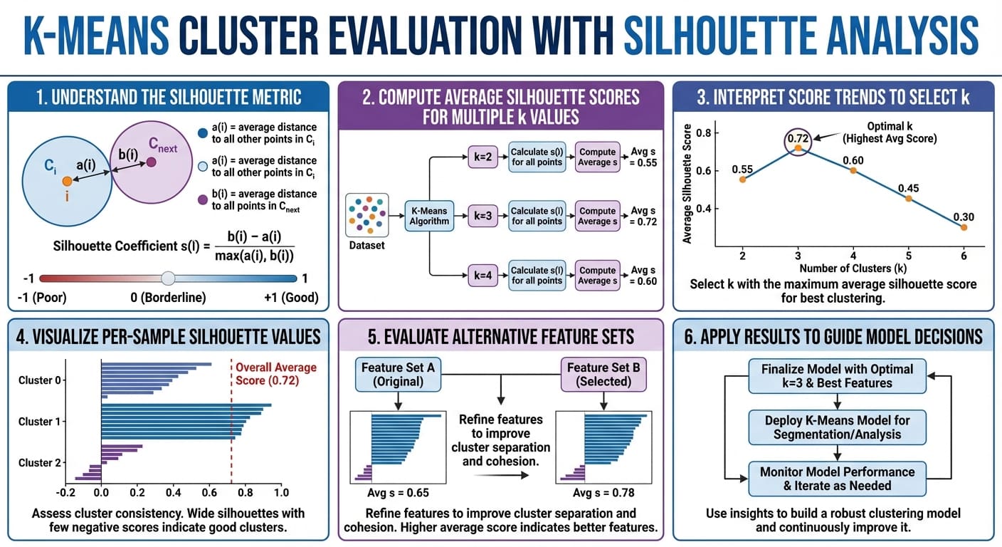
As you saw in the video, a silhouette plot shows:

Bars/Knives: Each colored bar represents a cluster.
Bar Height: The height indicates the number of data points in that cluster.
Bar Width: The width represents the silhouette scores of the points in that cluster. Wider is better.
Red Dashed Line: The average silhouette score for all data points.

When evaluating a plot, you are looking for:

High Average Score: The red dashed line should be as far to the right as possible.
Uniform Width: All clusters should ideally have scores above the average.
No Negative Scores: Bars extending to the left of zero signify points that are likely in the wrong cluster. This is a major sign of a poor fit.
Similar Thickness: The bars for each cluster should be of roughly similar thickness, indicating that the clusters are of a balanced size.

The following infographic provides an excellent summary of the entire silhouette analysis workflow.

K-Means Cluster Evaluation with Silhouette Analysis Infographic — This infographic summarizes the key steps of using Silhouette Analysis to evaluate a clustering model, from understanding the metric to using the results to make decisions.

Limitations of the Silhouette Score

While powerful, the silhouette score is not a perfect metric. It's important to be aware of its limitations to use it wisely.

Silhouette coefficient

Finally, to round out your understanding, let's review the drawbacks of this metric. The Hyperskill article provides a clear summary.

Read the short section titled 'Silhouette issues'.

The key limitations are:

Computational Cost: Its complexity is $O (n^{2})$ , making it slow for very large datasets.
Cluster Shape Assumption: It tends to favor convex, spherical clusters and may not perform well on clusters with complex shapes (e.g., elongated, or donut-shaped).
Curse of Dimensionality: It becomes less meaningful in very high-dimensional spaces because the concept of distance itself becomes less intuitive.

Conclusion

In this lesson, you've moved beyond simply using the silhouette score to pick a number and learned to use it as a sophisticated diagnostic tool. You can now quantitatively and visually assess the quality of a clustering solution.

Key Takeaways:

Clustering performance is evaluated based on cohesion (intra-cluster similarity) and separation (inter-cluster dissimilarity).
The silhouette score for a single point, $s_{i} = (b_{i} - a_{i}) / max (a_{i}, b_{i})$ , captures this trade-off. Scores range from -1 (misclassified) to +1 (ideal).
The Silhouette Coefficient is the average score across all points and provides a single metric for overall quality.
Silhouette plots offer a rich visual diagnosis, allowing you to check for misclassified points (negative scores), uneven cluster sizes, and clusters that are poorly separated.

Preview of the Next Lesson:
One of the key limitations we discussed is that the silhouette score (and k-means itself) struggles in high-dimensional space. In the next lesson, we will directly address this challenge by learning about dimensionality reduction. You will discover why reducing the number of features can be crucial for both visualization and improving model performance.

Recommended resources