K-Means Clustering: Implementation and Optimal K Selection

Implementing K-Means with Scikit-Learn

Let's dive into the implementation. We'll use Python's scikit-learn library, the standard toolkit for machine learning. This first video will walk you through a complete example, from loading data to applying the algorithm. As you watch, you'll notice a critical practical issue arise that wasn't obvious from our theoretical discussion.

The Importance of Feature Scaling

Did you notice the problem in the video? The clusters didn't look right. The green and black clusters were mixed up, even though our eyes can clearly separate the groups.

This is similar to the incorrect clustering result from the video. Notice how the vertical axis (income) has a much larger range than the horizontal axis (age), which distorts the distance calculations.

This happens because k-means relies on Euclidean distance. If one feature (like income) has a much larger scale than another (like age), the distance calculation will be dominated by the feature with the larger scale. The algorithm effectively ignores the feature with the smaller scale.

To fix this, we must normalize or standardize our features so they are on a comparable scale. A common technique is Min-Max scaling, which rescales each feature to a range between 0 and 1.

The next part of the video demonstrates exactly how to do this and shows the dramatically improved results.

This demonstrates a critical rule for distance-based algorithms like k-means: always scale your features before clustering.

Selecting the Optimal Number of Clusters (K)

In the example above, we could see three clusters just by looking at the scatter plot. But in most real-world scenarios, data has many dimensions and cannot be easily visualized. We need a quantitative way to choose the best value for $k$.

Method 1: The Elbow Method

The first technique we'll explore is the Elbow Method. The intuition is this: as we increase the number of clusters ($k$), the total WCSS (or inertia) will decrease. This is because with more clusters, each point will be closer to a centroid. At the extreme, if $k$ equals the number of data points, the inertia would be zero.

We are looking for the point where adding another cluster doesn't give us a significant decrease in inertia. This point on the plot looks like an "elbow" and is considered a good trade-off between model complexity (more clusters) and model fit (low inertia).

The Elbow Method is a useful heuristic, but sometimes the "elbow" is not very clear, making it hard to choose $k$ definitively.

Method 2: The Silhouette Score

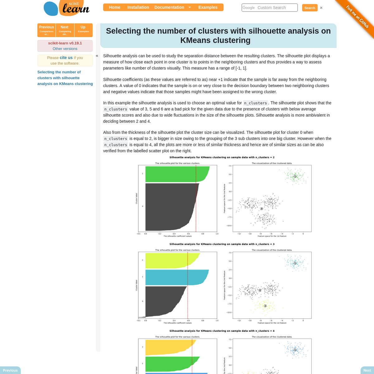
A more robust technique is the Silhouette Score. Unlike inertia, which only measures how compact a cluster is, the silhouette score measures both compactness (cohesion) and how well-separated a cluster is from other clusters (separation).

The score for a single data point is calculated as:

where:

• $a$: The average distance from the point to all other points in its own cluster.
• $b$: The average distance from the point to all points in the nearest neighboring cluster.

The score ranges from -1 to +1:

• +1: The point is far from other clusters and close to points in its own cluster (ideal).
• 0: The point is on or very close to the decision boundary between two clusters.
• -1: The point is likely assigned to the wrong cluster.

To find the optimal $k$, we calculate the average silhouette score for all data points for different values of $k$. The value of $k$ that gives the highest average silhouette score is considered the best.

Now, let's see how this is implemented and interpreted in practice.

The Complete Workflow

Let's summarize the full process for applying k-means clustering and selecting the best number of clusters.

1. Prepare the Data: Select the features you want to use for clustering.
2. Scale the Features: Use a scaler like StandardScaler or MinMaxScaler to bring all features to a comparable scale. This is a mandatory step.
3. Find the Optimal K:
   • Iterate through a range of possible $k$ values (e.g., 2 to 10).
   • For each $k$, fit a KMeans model on your scaled data.
   • Calculate and store the inertia_ for the Elbow Method plot.
   • Calculate and store the average silhouette_score for the Silhouette Plot.
4. Analyze the Plots:
   • Look for the "elbow" in the inertia plot.
   • Look for the peak in the silhouette score plot.
   • Choose the optimal $k$ that is suggested by one or both methods.
5. Build the Final Model: Instantiate and fit KMeans one last time using your chosen optimal $k$.
6. Analyze Results: You can now inspect the cluster assignments (.labels_) and the final centroids (.cluster_centers_) to understand the characteristics of each group.

The following resource provides a complete, end-to-end Python script following this workflow.

Conclusion

Congratulations! You have bridged the gap from k-means theory to practical implementation. You are now equipped to not only apply the algorithm but also to make a principled decision about its most important parameter, $k$.

Key Takeaways:

• You implement k-means in Python using the KMeans class from sklearn.cluster.
• Feature scaling is essential for distance-based algorithms like k-means to prevent features with large scales from dominating the result.
• The Elbow Method helps find an optimal $k$ by plotting inertia against the number of clusters and looking for the "elbow" point.
• The Silhouette Score is often a more reliable method. It measures both cluster cohesion and separation, and the optimal $k$ corresponds to the highest average score.
• The .fit_predict() method trains the model and returns cluster labels, while the inertia_ and cluster_centers_ attributes provide key information about the fitted model.

Preview of the Next Lesson:
In this lesson, we used the silhouette score as a tool to select the optimal number of clusters. In our next lesson, we will formalize its role as an evaluation metric to assess the quality of our final clustering solution and compare it with other potential models.