Training Neural Networks: Monitoring Loss and Accuracy

The Core Concepts of Training: Epochs and Batches

Before we press the "train" button, we need to understand two key parameters that control the training process: epochs and batch_size. These dictate how the model consumes the training data.

• An Epoch is one complete pass through the entire training dataset. If you have 10,000 training samples, one epoch is finished when the model has seen all 10,000 samples once.
• A Batch is a smaller subset of the training data. Instead of feeding all 10,000 samples to the network at once (which can be computationally expensive), we break them into smaller batches. The model's weights are updated after each batch is processed.

Think of it like studying for an exam. An epoch is like reading an entire textbook from cover to cover. A batch is like reading a single chapter, after which you pause to review and update your understanding.

To get a clear intuition for these concepts, please watch the following video segments.

If you have a dataset of 2,000 samples and a batch size of 100, it will take 20 batches (2000 / 100) to complete one epoch.

Executing the Training: model.fit()

With the concepts of epochs and batches understood, we can now look at the Keras function that puts them to use: model.fit(). This function orchestrates the entire training loop: it feeds batches of data to the model, triggers forward and backward passes, and updates the weights for a specified number of epochs.

When you call model.fit(), Keras performs the following loop:

1. For each epoch...
2. ...it iterates through the dataset in batches.
3. ...for each batch, it performs a forward pass, calculates the loss, performs backpropagation to get the gradients, and uses the optimizer to update the model's weights.
4. At the end of each epoch, it calculates the specified metrics (e.g., loss and accuracy) on the entire training set and prints them.

Monitoring Performance: The Key to Effective Training

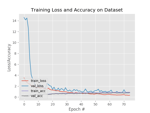
Watching the loss and accuracy numbers tick up is motivating, but it doesn't tell the whole story. A model can get a perfect score on its training data by simply memorizing it. This is called overfitting, and an overfit model will fail when presented with new, unseen data. True intelligence, whether human or artificial, is about the ability to generalize.

To check for generalization, we evaluate the model on a validation set (or test set)—data that it does not see during training.

• Training Loss/Accuracy: How well the model performs on the data it's learning from.
• Validation Loss/Accuracy: How well the model performs on new, unseen data. This is the true measure of its performance.

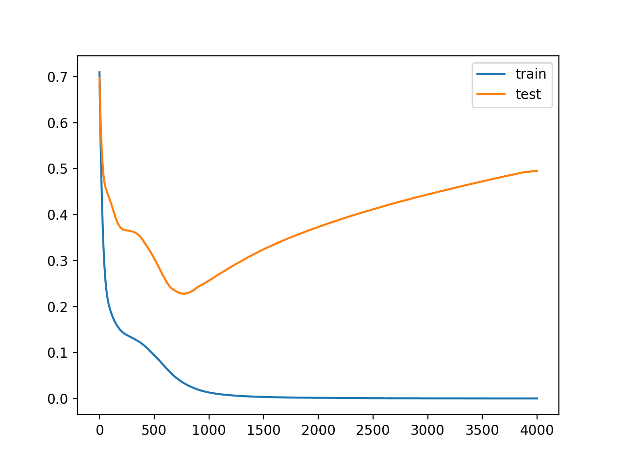
We aim for the validation loss to decrease along with the training loss. If the validation loss starts to increase while the training loss continues to decrease, it's a clear sign of overfitting.

The following video segment reinforces this crucial distinction.

Practical Implementation: Visualizing Training History

Keras makes it easy to monitor and visualize this process. The model.fit() function returns a History object, which contains a record of the loss and accuracy values at the end of each epoch for both the training and validation sets. We can then use a plotting library like Matplotlib to visualize these records.

Putting It All Together: A Complete Example

Let's integrate these concepts into a full code example. This script will:

1. Define and compile a simple model (like we did in the last lesson).
2. Train it on some data using model.fit(), using validation_split to create a validation set.
3. Capture the returned History object.
4. Plot the training and validation accuracy and loss over epochs.

import numpy as np
import matplotlib.pyplot as plt
from tensorflow.keras.models import Sequential
from tensorflow.keras.layers import Dense




# --- 1. Prepare Data (Example: Pima Indians Diabetes Dataset) ---
# For this example, we'll use a standard dataset.
# Make sure you have 'pima-indians-diabetes.csv' in the same directory.
# You can download it from: https://raw.githubusercontent.com/jbrownlee/Datasets/master/pima-indians-diabetes.data.csv
dataset = np.loadtxt("pima-indians-diabetes.csv", delimiter=",")
X = dataset[:,0:8]  # Input features (8 variables)
Y = dataset[:,8]   # Output class (0 or 1)




# --- 2. Build and Compile the Model ---
model = Sequential([
    Dense(12, input_shape=(8,), activation='relu'),
    Dense(8, activation='relu'),
    Dense(1, activation='sigmoid') # Sigmoid for binary classification
])

model.compile(
    loss='binary_crossentropy', 
    optimizer='adam', 
    metrics=['accuracy']
)




# --- 3. Train the Model ---
# We train for 150 epochs with a batch size of 10.
# `validation_split=0.33` tells Keras to hold out 33% of the data for validation.
print("Starting training...")
history = model.fit(
    X, 
    Y, 
    epochs=150, 
    batch_size=10, 
    validation_split=0.33,
    verbose=0 # verbose=0 silences the per-epoch output for a cleaner run
)
print("Training finished.")




# --- 4. Visualize Training History ---
# The history object contains the metrics recorded during training.
print("Plotting training history...")




# Plot training & validation accuracy values
plt.figure(figsize=(12, 5))
plt.subplot(1, 2, 1)
plt.plot(history.history['accuracy'])
plt.plot(history.history['val_accuracy'])
plt.title('Model Accuracy')
plt.ylabel('Accuracy')
plt.xlabel('Epoch')
plt.legend(['Train', 'Validation'], loc='upper left')




# Plot training & validation loss values
plt.subplot(1, 2, 2)
plt.plot(history.history['loss'])
plt.plot(history.history['val_loss'])
plt.title('Model Loss')
plt.ylabel('Loss')
plt.xlabel('Epoch')
plt.legend(['Train', 'Validation'], loc='upper left')

plt.tight_layout()
plt.show()

Run this code on your machine. The resulting plots are your primary tool for diagnosing how your model is learning. They give you the insight needed to decide what to do next.

Conclusion

Congratulations! You have now completed the entire core workflow of training a neural network: build, compile, and fit. You've moved from being an architect to being a coach, guiding the model's learning process and, crucially, monitoring its performance.

Key Takeaways:

• model.fit() is the function that trains your Keras model.
• Epochs define how many times the model sees the entire dataset.
• Batch size defines how many samples are processed before weights are updated.
• Monitoring validation metrics (val_loss, val_acc) is essential to assess generalization and detect overfitting.
• The History object returned by model.fit() stores the training metrics, which can be plotted to visualize the learning process.

Preview of the Next Lesson:
When you ran the code, you saw how the model performed with epochs=150 and batch_size=10. But are these the best choices? What about the learning rate in the 'adam' optimizer? These settings, which are not learned from the data but are set by you before training, are called hyperparameters. In our next lesson, "Tune key hyperparameters (learning rate, epochs, batch size) to improve model performance," we will explore how to systematically adjust these settings to squeeze the best possible performance out of your model.