Measures of Central Tendency and Dispersion

1. Measures of Central Tendency: The Mean

The most common way to find the "center" of a dataset is to calculate its mean, or average. However, in statistics, it's vital to distinguish between data that represents an entire population and data that is just a sample taken from that population.

• A population includes every member of a group of interest (e.g., all 240 billion cells in a biological experiment, every citizen of a country).
• A sample is a smaller, manageable subset of that population (e.g., a collection of 5 cells, a survey of 1000 citizens).

In AI and data science, you will almost always be working with samples, because collecting data for an entire population is usually impractical or impossible.

Let's watch a short video that clarifies the distinction between the population mean and the sample mean.

As the video explains, the formula is the same for both, but the notation and the conceptual meaning are different:

• Population Mean ($\mu$):

  $$\mu =\frac{{\sum }_{i=1}^N{x}_i}{N}$$

  where $N$ is the total number of items in the population.

• Sample Mean ($\bar{x}$):

  $$\bar{x}=\frac{{\sum }_{i=1}^n{x}_i}{n}$$

  where $n$ is the number of items in the sample.

The sample mean, $\bar{x}$, is our estimate of the true, often unknown, population mean, $\mu$.

2. Measures of Spread: Variance and Standard Deviation

The mean tells us where the center is, but it doesn't tell us anything about how the data is distributed around that center. For instance, two datasets could have the same mean but look completely different.

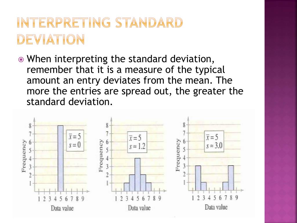
To quantify this spread, we use variance and standard deviation.

Why do we need a new measure?

Our first impulse might be to calculate the average distance of each point from the mean, $(x_i-\mu )$. However, the positive differences and negative differences would cancel each other out, always summing to zero.

To solve this, we square each difference, making all the values positive. This gives larger weight to points that are farther from the mean.

Variance

Variance is defined as the average of the squared differences from the mean.

• Population Variance (${\sigma }^2$): $${\sigma }^2=\frac{{\sum }_{i=1}^N(x_i-\mu {)}^2}{N}$$

One issue with variance is that its units are squared (e.g., if you measure height in meters, the variance is in meters-squared). This makes it difficult to interpret directly in the context of the original data.

Standard Deviation

Standard Deviation solves the units problem. It is simply the square root of the variance. This brings the measure of spread back into the original units of the data.

• Population Standard Deviation ($\sigma$): $$\sigma =\sqrt{\frac{{\sum }_{i=1}^N(x_i-\mu {)}^2}{N}}$$

The standard deviation gives us a "standard" or "typical" measure of how far a data point is from the mean.

A Small but Crucial Change for Samples

When we calculate the variance from a sample, we have to make a small adjustment. We are using the sample mean $\bar{x}$ as an estimate of the true population mean $\mu$. It turns out that this leads to a slight underestimation of the true population variance.

To correct for this, we divide by n-1 instead of n. This is known as Bessel's correction.

• Sample Variance ($s^2$):

  $$s^2=\frac{{\sum }_{i=1}^n(x_i-\bar{x}{)}^2}{n-1}$$

• Sample Standard Deviation ($s$):

  $$s=\sqrt{\frac{{\sum }_{i=1}^n(x_i-\bar{x}{)}^2}{n-1}}$$

This is a critical point: In almost all practical applications in AI, you will use the sample formulas (dividing by n-1).

Let's watch the rest of the StatQuest video to see these concepts explained with clear visuals and formulas.

The image below summarizes the formulas for sample calculations, which you will use most often.

3. Calculation and Interpretation in Practice

Now let's solidify this by working through an example and focusing on interpretation.

Let's recap the steps from the resource for the dog heights dataset {600, 470, 170, 430, 300}:

1. Calculate the Mean ($\mu$):
   $\mu =(600+470+170+430+300)/5=394$ mm.

2. Calculate Squared Differences from the Mean:

   • $(600-394{)}^2=206^2=42,436$
   • $(470-394{)}^2=76^2=5,776$
   • $(170-394{)}^2=(-224{)}^2=50,176$
   • $(430-394{)}^2=36^2=1,296$
   • $(300-394{)}^2=(-94{)}^2=8,836$

3. Calculate the Variance (${\sigma }^2$):
   Average the squared differences (dividing by N=5 for population):
   ${\sigma }^2=(42436+5776+50176+1296+8836)/5=108,520/5=21,704$ mm${}^2$.

4. Calculate the Standard Deviation ($\sigma$):
   Take the square root of the variance:
   $\sigma =\sqrt{21704}\approx 147.3$ mm.

Interpretation: The mean height is 394 mm, and the standard deviation is about 147 mm. This tells us that a typical dog in this group has a height that is roughly 147 mm away from the average height.

Now, if these 5 dogs were just a sample of a larger population of dogs, the only change would be in step 3:

3. Calculate the Sample Variance ($s^2$):
   Divide by n-1 = 4:
   $s^2=108,520/4=27,130$ mm${}^2$.

4. Calculate the Sample Standard Deviation ($s$):
   $s=\sqrt{27130}\approx 164.7$ mm.

Notice that the sample standard deviation is slightly larger. This is the result of Bessel's correction, giving us a more accurate estimate of the spread in the larger, unseen population.

What Does It Mean in the Real World?

A small standard deviation means data points are clustered tightly around the mean, implying consistency and predictability. A large standard deviation means data points are spread out, implying inconsistency.

To see why this is so important, read this practical example.

The pizza example shows that even if two models, systems, or processes have the same average performance (mean), the one with lower standard deviation is often more reliable and desirable because its outcomes are more consistent.

Conclusion

In this lesson, you've learned to compute and interpret three foundational statistics. These measures provide a concise summary of a dataset's central tendency and spread, which is a fundamental skill for any work in data science and AI.

Key Takeaways:

• The mean ($\mu$ or $\bar{x}$) gives the central or average value of a dataset.
• Variance (${\sigma }^2$ or $s^2$) measures the average squared distance from the mean. It's mathematically convenient but uses squared units.
• Standard Deviation ($\sigma$ or $s$) is the square root of the variance. It measures the typical or standard spread of data points around the mean, in the original units of the data.
• When working with a sample of data (which is almost always the case), we divide by n-1 when calculating variance to get a better estimate of the true population variance.

Preview of the Next Lesson:
The standard deviation is a powerful tool on its own, but its true power is unlocked when combined with knowledge about the shape of the data's distribution. In our next lesson, we will focus on the most famous distribution of all: the normal distribution (or "bell curve"). You will learn about its properties and see how the mean and standard deviation allow us to make remarkably accurate predictions about the data.