Discrete vs. Continuous Random Variables

1. The Fundamental Distinction: Counting vs. Measuring

At its core, the difference between discrete and continuous random variables is the difference between counting and measuring.

• Discrete random variables are typically the result of counting. They can only take on a finite or countably infinite number of distinct values. There are "gaps" between the possible values.
• Continuous random variables are typically the result of measuring. They can take on any value within a given range. There are no gaps between the possible values; between any two values, there is always another possible value.

To build a strong intuition for this, let's watch a video that explores this distinction with several clear examples.

As the video highlighted, think about these key questions when classifying a random variable:

• Can I list all the possible outcomes, even if that list is infinite? (e.g., 0, 1, 2, 3, ...). If yes, it's discrete.
• Does the variable represent a measurement that could be infinitely precise, taking any value in a range? (e.g., height, weight, time). If yes, it's continuous.

2. Describing Distributions: PMF, PDF, and CDF

Now that we can distinguish between the two types of variables, how do we describe their associated probabilities? For example, how do we state the probability of a fair die landing on '3' versus the probability of a person's height being exactly 175cm? The approaches are fundamentally different.

This brings us to the concept of probability distributions, which are functions that describe the likelihood of a random variable taking on certain values.

Let's summarize the key functions from the video:

• Probability Mass Function (PMF):

  • Used for discrete random variables.
  • Assigns a specific probability to each possible value. For a random variable $X$, the PMF gives $P(X=x)$.
  • The sum of all probabilities in a PMF must equal 1.
  • Example: For a fair six-sided die, the PMF would be $P(X=x)=1/6$ for $x\in \{1,2,3,4,5,6\}$.

• Probability Density Function (PDF):

  • Used for continuous random variables.
  • The value of the PDF at a point, $f(x)$, is not a probability. It represents a "probability density."
  • Probabilities are found by calculating the area under the curve of the PDF over an interval. The probability of $X$ falling between $a$ and $b$ is ${\int }_a^{b}f(x)dx$.
  • This implies that the probability of a continuous random variable being exactly a specific value is zero: $P(X=x)={\int }_x^{x}f(t)dt=0$. This is a crucial, though sometimes counter-intuitive, point.
  • The total area under the entire PDF curve must equal 1.

• Cumulative Distribution Function (CDF):

  • Can be used for both discrete and continuous random variables.
  • It gives the cumulative probability of the random variable being less than or equal to a value $x$. That is, $F(x)=P(X\le x)$.
  • For a discrete variable, the CDF is a step function.
  • For a continuous variable, the CDF is a smooth, non-decreasing function that goes from 0 to 1.

The connection to calculus is powerful: the PDF is the derivative of the CDF, and the CDF is the integral of the PDF. This gives you a formal way to move between these two representations.

3. Formalizing the Concepts

The videos provided a great intuitive and visual understanding. Now, let's solidify these ideas with more formal definitions, which are essential for applying these concepts rigorously in AI and machine learning.

This reading reinforces the key ideas we've covered. The probability of a continuous random variable taking on any single, exact value is zero because there are infinitely many possible values. Think of it like a dart hitting a board, as described in the textbook Dive into Deep Learning. The chance of hitting a single mathematical point is zero; you can only talk about the probability of hitting a certain area. Similarly, for a continuous random variable, we can only talk about the probability of it falling within a certain interval.

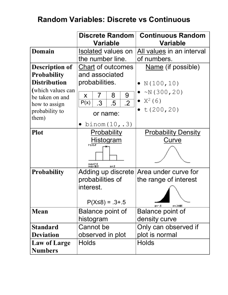
4. Summary Table

To consolidate your understanding, here is a helpful table that summarizes the key distinctions between discrete and continuous random variables.

Conclusion

In this lesson, you've learned the critical distinction between discrete and continuous random variables and how their probability distributions are described. This is not just a theoretical exercise; choosing the correct type of distribution is a fundamental step in building probabilistic models in AI. For example, a model predicting customer churn (a yes/no outcome) would use a discrete distribution, while a model predicting house prices would use a continuous one.

Key Takeaways:

• Discrete Random Variables are countable (e.g., number of coin flips) and are described by a Probability Mass Function (PMF), which gives the probability at each distinct point.
• Continuous Random Variables are measurable (e.g., height, time) and are described by a Probability Density Function (PDF), where probability is the area under the curve over an interval.
• For any continuous variable $X$, the probability of it taking an exact value is zero, i.e., $P(X=x)=0$.
• The Cumulative Distribution Function (CDF), $F(x)=P(X\le x)$, is a unifying concept that applies to both types of variables and represents the total accumulated probability up to a value $x$.

Preview of the Next Lesson:
Simply knowing the distribution of a variable isn't always enough. We often want to summarize its main characteristics in just a few numbers. In the next lesson, you will learn how to compute and interpret mean, variance, and standard deviation for a dataset. We will see how the calculation of these summary statistics depends on whether the variable is discrete or continuous, building directly on the foundations you've established today.