Conditional Probability and Bayes' Theorem

Introduction

Welcome back to our module on Probability and Statistics for AI. In the last lesson, you learned the fundamental rules for combining probabilities of events, focusing on the addition rule ("OR") and the multiplication rule ("AND"). A key assumption for the simple multiplication rule, $P (A \cap B) = P (A) \times P (B)$ , was that the events A and B are independent.

However, in the real world, events are rarely independent. The probability of traffic being bad is not independent of whether it's raining. In AI, a system's "belief" that an email is spam should change based on the "evidence" that it contains the word "lottery."

Today, we will address this by learning to compute conditional probabilities and apply Bayes' theorem to update beliefs. This lesson is a crucial step toward your goal of building intelligent systems, as Bayes' theorem is the mathematical engine that allows a model to learn from data and rationally update its understanding of the world.

1. When Events Depend on Each Other: Conditional Probability

Let's start by formalizing the idea of dependent events. If the occurrence of one event affects the probability of another, we need the concept of conditional probability.

The conditional probability of event A occurring given that event B has already occurred is written as $P (A ∣ B)$ . Think of it as a recalculation of probability within a new, smaller sample space defined by event B.

Conditional probability

This document, 'Conditional probability' from UConn's probability course, provides a clear, formal definition of conditional probability and the general multiplication rule that arises from it.

Read the first page of the document, up to and including 'Example 4.3'. Focus on the definition of P(E|F) and how it's used in the examples with dice and marbles. This formalizes the idea of a restricted sample space.

The definition you just read is:

P (A ∣ B) = \frac{P ( A \cap B )}{P ( B )}

This states that the probability of A given B is the ratio of the probability of both A and B happening to the probability of B happening.

By rearranging this formula, we get the General Multiplication Rule, which works for any two events, dependent or not:

P (A \cap B) = P (A ∣ B) P (B)

Notice that if A and B are independent, then by definition $P (A ∣ B) = P (A)$ , and this rule simplifies back to the $P (A \cap B) = P (A) P (B)$ that you learned in the previous lesson.

2. Introducing Bayes' Theorem: A Formula for Updating Beliefs

The General Multiplication Rule has a symmetric counterpart: $P (A \cap B) = P (B ∣ A) P (A)$ . Since both expressions are equal to $P (A \cap B)$ , we can set them equal to each other:

P (A ∣ B) P (B) = P (B ∣ A) P (A)

Dividing by $P (B)$ gives us the famous Bayes' Theorem:

P (A ∣ B) = \frac{P ( B ∣ A ) P ( A )}{P ( B )}

This simple algebraic rearrangement is one of the most powerful ideas in statistics and AI. It allows us to "flip" a conditional probability. Often, we know how likely we are to see some evidence given a certain hypothesis (e.g., the probability of a positive test result given you have a disease), but what we really want to know is the probability of the hypothesis given the evidence (the probability you have the disease given a positive test).

Bayes' Theorem of Probability With Tree Diagrams & Venn Diagrams

To see this derivation in action, watch this short introductory clip from The Organic Chemistry Tutor.

Watch the first 2 minutes and 28 seconds of the video 'Bayes' Theorem of Probability With Tree Diagrams & Venn Diagrams'. This will walk you through the exact algebraic steps we just took to derive the formula.

3. The Intuition Behind Updating Beliefs

A formula is one thing, but to build a "superpower brain" for decision-making, you need a deep, intuitive grasp of why it works. The core idea behind Bayes' theorem is that evidence should update prior beliefs, not replace them. Our intuition often fails us here.

Let's explore this with a classic thought experiment.

Bayes theorem, the geometry of changing beliefs

This brilliant video from 3Blue1Brown, 'Bayes theorem, the geometry of changing beliefs', uses a psychological puzzle to show how our minds often misinterpret evidence and how Bayesian reasoning corrects this error.

Watch the segment from 01:04 to 04:46. Pay close attention to the 'Steve the librarian/farmer' example. The key is to realize that the description of Steve (the evidence) must be weighed against the initial ratio of farmers to librarians (the prior belief).

The error most people make is ignoring the prior probability (or base rate)—the fact that there are far more farmers than librarians to begin with. The correct approach, as the video shows, is to:

Start with a representative sample based on your prior beliefs (e.g., 200 farmers, 10 librarians).
Apply the evidence to see how many from each group fit the description (e.g., 20 farmers and 4 librarians).
Calculate the new probability from this restricted group (4 out of 24 total are librarians).

This process of updating is exactly what Bayes' theorem formalizes.

4. Decoding the Formula and Visualizing It

Now, let's map the intuitive steps from the video onto the formal theorem. In Bayesian terms, we are calculating the probability of a Hypothesis (H) given some Evidence (E).

The formula is:

P (H ∣ E) = \frac{P ( E ∣ H ) \cdot P ( H )}{P ( E )}

Let's watch how the video connects this formula to the "Steve" example.

Bayes theorem, the geometry of changing beliefs

This next segment breaks down the formula, assigning specific names to each part, and introduces a powerful geometric way to visualize the theorem.

Watch from 04:46 to 10:18. Focus on understanding the meaning of each term: Posterior, Likelihood, and Prior. Also, grasp the area-based diagram; it's a flexible mental model for solving Bayesian problems.

Here is a summary of the terminology:

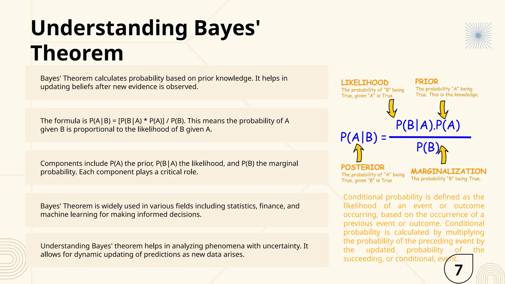
Understanding Bayes' Theorem — Bayes' Theorem provides a principled way to update our beliefs. The posterior probability is what we compute, based on our prior belief, the likelihood of evidence, and the marginal probability of that evidence.

$P (H ∣ E)$ is the Posterior: The updated probability of the hypothesis after seeing the evidence. This is what we want to calculate.
$P (H)$ is the Prior: The initial probability of the hypothesis before seeing the evidence (e.g., the base rate of librarians).
$P (E ∣ H)$ is the Likelihood: The probability of seeing the evidence if the hypothesis is true (e.g., the probability a person fits Steve's description, given they are a librarian).
$P (E)$ is the Marginal Likelihood / Evidence: The overall probability of seeing the evidence, averaged over all hypotheses.

The denominator, $P (E)$ , is often the trickiest part. We calculate it using the Law of Total Probability:

P (E) = P (E ∣ H) P (H) + P (E ∣ H^{c}) P (H^{c})

This means the total probability of the evidence is the sum of: (the probability of the evidence if the hypothesis is true, weighted by the prior) + (the probability of the evidence if the hypothesis is false, weighted by its prior).

5. Applying Bayes' Theorem: A Medical Diagnosis Problem

Let's put this all together to solve a classic, practical problem. This type of calculation is critical in fields from medical diagnostics to spam filtering in AI.

Problem: A certain disease affects 1% of the population. A test for the disease is 95% accurate (i.e., if you have the disease, it correctly returns positive 95% of the time). The test also has a 2% false positive rate (i.e., if you don't have the disease, it incorrectly returns positive 2% of the time). If a randomly chosen person tests positive, what is the probability they actually have the disease?

Before you see the solution, try to guess. Is it around 95%?

Now, let's use Bayesian reasoning to find the real answer.

Bayes' Theorem of Probability With Tree Diagrams & Venn Diagrams

The Organic Chemistry Tutor provides an exceptionally clear, step-by-step solution to a very similar medical diagnosis problem. The video demonstrates two powerful methods for solving it.

Watch from 08:32 to 19:05. First, follow the tree diagram method, which is a great way to organize the probabilities to calculate the denominator P(Positive Test). Then, pay close attention to the second method using a hypothetical population (e.g., 10,000 people). This 'natural frequencies' approach is often more intuitive and less error-prone than plugging numbers into a formula.

Let's recap the steps for our specific problem:

Hypothesis (H): The person has the disease.
Evidence (E): The person tests positive.
Prior $P (H)$ : 0.01 (1% of the population has the disease).
Likelihood $P (E ∣ H)$ : 0.95 (the test is 95% accurate for sick people).
False Positive Rate $P (E ∣ H^{c})$ : 0.02 (2% of healthy people test positive).

First, we calculate the total probability of testing positive, $P (E)$ :

P (E) = P (E ∣ H) P (H) + P (E ∣ H^{c}) P (H^{c})

P (E) = (0.95 \times 0.01) + (0.02 \times 0.99) = 0.0095 + 0.0198 = 0.0293

Now, we apply Bayes' theorem:

P (H ∣ E) = \frac{P ( E ∣ H ) P ( H )}{P ( E )} = \frac{0.95 \times 0.01}{0.0293} = \frac{0.0095}{0.0293} \approx 0.324

The actual probability of having the disease is only about 32.4%! This is often surprising, but it makes sense when you realize that false positives from the large healthy population (99%) contribute more positive tests than true positives from the small sick population (1%). This is a perfect example of Bayesian reasoning providing a counter-intuitive but correct answer, a true "superpower" for rational decision-making.

Conclusion

In this lesson, you've moved beyond simple probabilities to tackle dependent events and the powerful logic of belief updating. This is a cornerstone of modern AI.

Key Takeaways:

Conditional Probability $P (A ∣ B)$ allows us to reason about events when the outcome of one affects the other.
Bayes' Theorem is a direct consequence of conditional probability that gives us a mathematical rule for updating our beliefs ( $P (H)$ , the prior) in light of new information ( $E$ , the evidence) to arrive at a more informed belief ( $P (H ∣ E)$ , the posterior).
The formula $P (H ∣ E) = \frac{P ( E ∣ H ) P ( H )}{P ( E )}$ is used across AI for tasks like classification, diagnosis, and filtering.
Intuitive methods like tree diagrams and natural frequencies (hypothetical populations) are powerful tools for solving Bayesian problems correctly.

Preview of the Next Lesson:
So far, we've talked about the probability of discrete events (e.g., "rolling a 6," "testing positive"). To build more powerful AI models, we need to handle numerical outcomes, such as predicting a price or a temperature. In the next lesson, you will learn to distinguish between discrete and continuous random variables and their distributions. This will provide the framework for describing and modeling the numerical outputs of probabilistic systems.

Recommended resources