Understanding the Normal Distribution

1. What is the Normal Distribution?

The normal distribution is a continuous probability distribution that describes a vast number of phenomena in nature and society. From human height and blood pressure to measurement errors in an experiment, data often tends to cluster around a central value with no bias to the left or right.

Let's begin by building an intuition for this pattern.

As the video shows, the normal distribution is defined by its characteristic shape:

• It is symmetrical around a central peak.
• The data values are most frequent around this central peak.
• The frequency of values tapers off as you move further away from the center.
• The curve is unimodal, meaning it has only one peak.

The significance of a distribution's graph is that it shows us which values are common (where the curve is high) and which are rare (where the curve is low). For the normal distribution, this means values near the center are typical, while extreme values are progressively less likely.

2. The Defining Parameters: Mean and Standard Deviation

Here is where our previous lesson connects directly to today's topic. A remarkable property of the normal distribution is that its entire shape and all of its probabilities are completely defined by just two parameters:

1. The Mean ($\mu$): This determines the location of the center or peak of the curve. Changing the mean shifts the entire curve left or right along the x-axis.
2. The Standard Deviation ($\sigma$): This determines the spread or width of the curve. A small standard deviation results in a tall, narrow curve (data is tightly clustered around the mean), while a large standard deviation results in a short, wide curve (data is spread out).

Let's see this in action.

The image below provides a fantastic summary of all the key properties of the normal distribution we've discussed so far.

3. The Empirical Rule: A Practical Tool

Now that you know the curve is defined by $\mu$ and $\sigma$, we can introduce a powerful rule of thumb called the Empirical Rule (or the 68-95-99.7 rule). This rule tells us the approximate percentage of data that falls within a certain number of standard deviations from the mean in any normal distribution.

Specifically, for a normal distribution:

• Approximately 68% of the data falls within 1 standard deviation of the mean ($\mu \pm 1\sigma$).
• Approximately 95% of the data falls within 2 standard deviations of the mean ($\mu \pm 2\sigma$).
• Approximately 99.7% of the data falls within 3 standard deviations of the mean ($\mu \pm 3\sigma$).

This rule is incredibly useful because it allows us to quickly estimate the range that contains the vast majority of our data, just by knowing the mean and standard deviation.

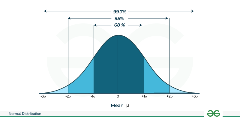
Let's apply this. Consider the pizza delivery example from the statisticsbyjim.com article you saw in the last lesson. If a pizza restaurant's delivery times are normally distributed with a mean ($\mu$) of 30 minutes and a standard deviation ($\sigma$) of 5 minutes:

• We can expect about 68% of deliveries to be between 25 and 35 minutes (30 ± 5).
• We can expect about 95% of deliveries to be between 20 and 40 minutes (30 ± 2*5).
• Almost all (99.7%) deliveries will be between 15 and 45 minutes (30 ± 3*5).

A delivery time of 50 minutes would be four standard deviations from the mean ($(50-30)/5=4$), making it a very rare event (outside the 99.7% range).

4. The Mathematical Foundation

Given your theory-first preference and your goal to achieve deep understanding, it's valuable to see the mathematical engine that generates this beautiful curve. The shape of the normal distribution is described by a Probability Density Function (PDF).

For a random variable $X$ that follows a normal distribution with mean $\mu$ and variance ${\sigma }^2$, denoted as $X\sim N(\mu ,{\sigma }^2)$, its PDF is:

You don't need to memorize this formula, but you should appreciate what it represents:

• It is a precise mathematical function that draws the bell curve.
• The inputs to the function are the data value $x$, the mean $\mu$, and the standard deviation $\sigma$. This confirms that $\mu$ and $\sigma$ are the sole parameters that define the distribution.
• The term $\frac{x-\mu }{\sigma }$ is the distance of a point from the mean, measured in units of standard deviation. This value, called a z-score, is central to working with normal distributions, as we will see later.

5. The Significance of the Normal Distribution

Why is this one distribution so important? Its significance stems from a few key facts.

Let's summarize and expand on the key points from the reading:

1. It Models the World: As we've seen, many natural and engineered processes produce data that is normally distributed. This makes it an excellent model for real-world phenomena.

2. It is a Foundation for Statistical Inference: Many statistical hypothesis tests, which are used to make decisions from data (e.g., "Is my new AI model better than the old one?"), assume that the data or errors in the model follow a normal distribution.

3. The Central Limit Theorem (CLT): This is perhaps the most profound reason for the normal distribution's importance. The CLT states that if you take sufficiently large samples from any population (even a non-normal one) and calculate the mean of each sample, the distribution of those sample means will be approximately normal. This is a powerful, almost magical result that makes the normal distribution the cornerstone of statistical theory.

Conclusion

In this lesson, you explored the fundamental properties and immense significance of the normal distribution. It is far more than just a bell-shaped curve; it's a key to understanding variability and making predictions about data.

Key Takeaways:

• The normal distribution is a symmetric, unimodal, bell-shaped curve that models countless real-world phenomena.
• Its shape is entirely determined by two parameters: the mean ($\mu$), which sets its location, and the standard deviation ($\sigma$), which sets its spread.
• The Empirical Rule (68-95-99.7) provides a powerful shortcut to estimate the percentage of data within 1, 2, and 3 standard deviations of the mean.
• Its significance in AI and statistics comes from its ability to model data, its role in hypothesis testing, and most importantly, the Central Limit Theorem.

Preview of the Next Lesson:
We briefly introduced the Central Limit Theorem as the "magical" reason for the normal distribution's ubiquity. In the next lesson, we will explore this theorem in detail. You will learn what a sampling distribution is and see how the CLT allows us to make powerful inferences about an entire population using just a single sample. This is a critical step toward understanding how statistical testing and machine learning models work.