One-at-a-Time Sensitivity Analysis for Multi-variable Models

The One-at-a-Time (OAT) Framework

The OAT method is the most intuitive form of LSA. As its name implies, it involves changing one input factor at a time while holding all others constant to observe the effect on the model's output.

The OAT procedure can be systemized into a clear, repeatable algorithm:

1. Establish a Base Case: Define a baseline scenario by setting all input parameters to their nominal or expected values. Calculate the model's output for this base case.
2. Perturb One Input: Select one input parameter and change its value by a specific amount (e.g., +10% or +1 standard deviation), while keeping all other parameters fixed at their base-case values.
3. Measure the Impact: Calculate the new model output and record the deviation from the base-case output.
4. Repeat: Revert the change from the previous step and repeat the process for every other input parameter, one by one.
5. Rank: Compare the magnitude of the output deviations caused by each input perturbation. Rank the parameters from most to least influential.

This process is often visualized using a tornado chart, which provides an immediate visual ranking of parameter sensitivities.

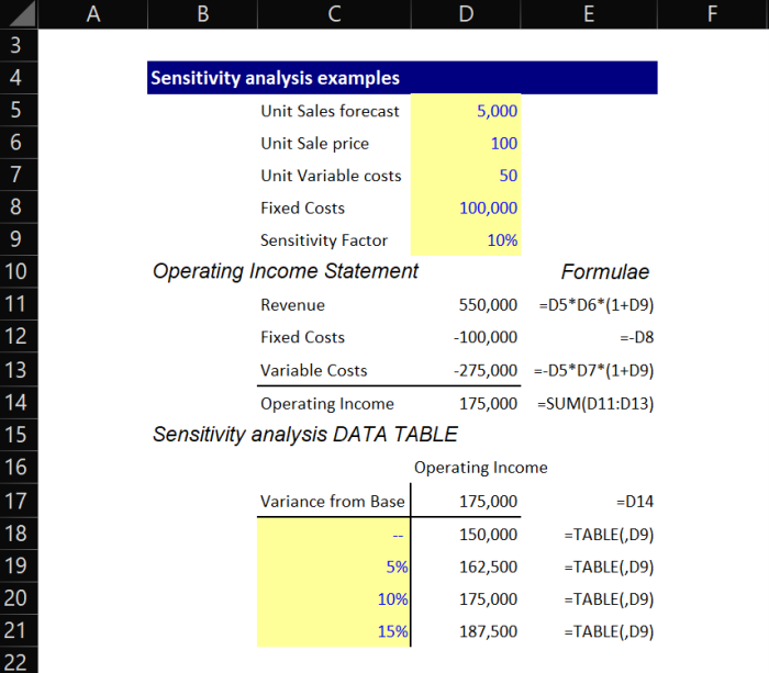
Case Study: A Profit Maximization Model

To make this procedure concrete, we'll use a clear, multi-variable optimization problem.

Let's summarize the model and establish our base case. The profit $P$ as a function of time $t$ (in days) is given by:

With the specific parameters from the video, this becomes:

The video determines that the optimal time to sell is $t^{\ast }=8$ days, which yields a maximum profit of $P(8)=\$133.20$. This is our base case.

Our model has several input parameters we can analyze:

• Initial weight: 200 lbs
• Growth rate (g): 5 lbs/day
• Initial price: $0.65/lb
• Rate of price fall (r): $0.01/lb/day
• Daily keeping cost: $0.45/day

We want to answer: Which of these parameters has the biggest impact on the maximum profit?

Executing the OAT Analysis

We will now perturb two of these parameters—the growth rate g and the rate of price fall r—to quantify their influence.

Quantifying and Ranking Sensitivity

The video demonstrates the process, but to rank parameters, we need a standardized sensitivity metric. We'll explore two methods.

Method 1: The Normalized Derivative (Elasticity)

For a mathematically rigorous approach, we can approximate the partial derivative of the output with respect to each input. The sensitivity index $S_i$ for an input $x_i$ on output $g(x)$ is often defined using a finite difference approximation:

To compare parameters with different units (e.g., lbs/day vs. $/lb/day), we normalize this derivative to calculate elasticity—the percentage change in output for a percentage change in input.

A higher absolute value of this metric indicates greater sensitivity.

The video calculates this directly for the profit's sensitivity to the growth rate.

So, for the growth rate g, the sensitivity is 0.17.

Let's perform this calculation for the rate of price fall, r.

1. Base Case: r = 0.01, t* = 8, P_max = $133.20.
2. Perturb: Let's increase r by 10% to r' = 0.011.
3. Find new optimum: As derived in the video, the optimal time is a function of r: $T(r)=\frac{7-500r}{25r}$. For r' = 0.011, the new optimal time is $t^{\prime }=\frac{7-500(0.011)}{25(0.011)}\approx 5.45$ days.
4. Calculate new max profit: We must use the new parameter r' and the new time t' in the profit function: $$P(t^{\prime },r^{\prime })=(0.65-r^{\prime }{t}^{\prime })(200+5t^{\prime })-0.45t^{\prime }$$ $$P(5.45,0.011)=(0.65-0.011\times 5.45)(200+5\times 5.45)-0.45\times 5.45\approx \$131.64$$
5. Calculate Sensitivity: $$\%\Delta P=\frac{131.64-133.20}{133.20}\approx -1.17\%$$ $${\text{Sensitivity}}_r=\frac{\%\Delta P}{\%\Delta r}=\frac{-1.17\%}{+10\%}=-0.117$$

Method 2: Direct Percentage Change

For many screening purposes, a simpler "brute force" calculation is sufficient. You simply calculate the percentage change in the output resulting from a fixed percentage change (e.g., +10%) in the input. This is essentially the numerator of the elasticity calculation.

• For g: A +10% change in g resulted in a +1.7% change in profit.
• For r: A +10% change in r resulted in a -1.17% change in profit.

Ranking the Factors

Now we can rank these two factors based on the absolute magnitude of their impact.

Our OAT analysis shows that the maximum profit is more sensitive to the pig's growth rate (g) than to the rate at which the market price falls (r). A 10% improvement in growth rate yields a greater return than a 10% improvement (i.e., reduction) in the rate of price decline. If we were to continue this for all five parameters, we would generate a complete ranked list.

Conclusion

You have now moved from the concept of local sensitivity analysis to its practical execution. You have learned a systematic, quantitative procedure to test the influence of each input variable in a model and, crucially, how to rank them. This process is the foundation of quantitatively identifying your primary bottleneck or 'Hook'.

Key Takeaways:

• One-at-a-Time (OAT) analysis follows a clear algorithm: establish a base case, perturb inputs individually, measure the output change, and rank the results.
• To compare the influence of different parameters, a normalized sensitivity metric like elasticity (%ΔOutput / %ΔInput) is used.
• The final output of an OAT analysis is a ranked list of input factors, ordered from most to least influential on the model's output.

Preview of the Next Lesson:

Our OAT analysis has given us a ranked list of influential factors. However, in most complex systems, a small number of factors are responsible for the vast majority of the effect. How do we formally separate these "vital few" from the "trivial many"? In the next lesson, we will apply Pareto (80/20) analysis to isolate the vital few factors from the trivial many in a system, allowing you to focus your strategic efforts where they will have the greatest impact.