Local vs. Global Sensitivity Analysis

Introduction

In our last lesson, we established a method for deconstructing a complex goal, like achieving high output in scientific research, into a resource-dependency map. We framed this using a multiplicative model, Output ≈ α_Funding × α_Quality × ..., where the 'Hook' or primary constraint is the factor with the lowest performance. This gave us a conceptual framework to identify the bottleneck.

Today, we move from the conceptual to the quantitative. Your goal is not just to guess the 'Hook', but to prove its identity and quantify its impact. The tool for this is Sensitivity Analysis (SA). This lesson will introduce the two primary families of SA: local and global methods. Your learning outcome is to differentiate between these two approaches, understanding their distinct methodologies, scopes, and limitations. This foundational knowledge is critical for selecting the right analytical tool for any given system.

What is Sensitivity Analysis?

At its core, sensitivity analysis is the study of how uncertainty in the output of a mathematical model can be apportioned to different sources of uncertainty in its inputs. In the context of your P_max model, it answers the question: "If I could improve one of my input factors (Time, Skill, etc.), which one would give me the biggest boost in my final output?"

Let's begin with a concise overview of the purpose and value of sensitivity analysis.

04 1 Local Sensitivity Analysis

This video, titled 'Local Sensitivity Analysis' by Jef Karel Caers, provides a clear introduction to the concept of sensitivity analysis in general.

Watch from 00:22 to 03:06. Focus on the three key purposes of SA mentioned: Reducing uncertainty in predictions. Reducing the complexity of a problem. Understanding the effect of parameter combinations and interactions.

The Two Families of Sensitivity Analysis

As the video briefly introduces, SA methods can be broadly divided into two categories: local and global. The choice between them is not arbitrary; it depends on the complexity of your model and the nature of the questions you are asking.

The following video segment draws a sharp, immediate distinction between the two approaches.

04 1 Local Sensitivity Analysis

Continuing with the same resource, this section directly contrasts the fundamental approaches of local and global sensitivity analysis.

Watch from 03:06 to 04:08. Pay close attention to the core difference: local SA starts from a 'base case' and perturbs it, while global SA explores the entire parameter space without a privileged base case.

Let's dissect these two approaches with more precision.

Local Sensitivity Analysis (LSA): The "What-If" at a Point

Local Sensitivity Analysis investigates the model's response to small perturbations of its inputs around a single, fixed point in the input space (the "base case").

From a mathematical perspective, which will be familiar to you, LSA is fundamentally about calculating the local gradient of the output function with respect to its inputs. The local sensitivity of an output $Y = g (X_{1}, X_{2}, ..., X_{k})$ to an input $X_{i}$ is simply its partial derivative at a specific point $X^{*}$ :

S_{i} = \frac{\partial g ( X )}{\partial X _{i}}_{X = X^{*}}

The most common and intuitive method of LSA is One-at-a-Time (OAT) analysis. You hold all inputs constant at their base-case values and vary a single input to observe its effect on the output.

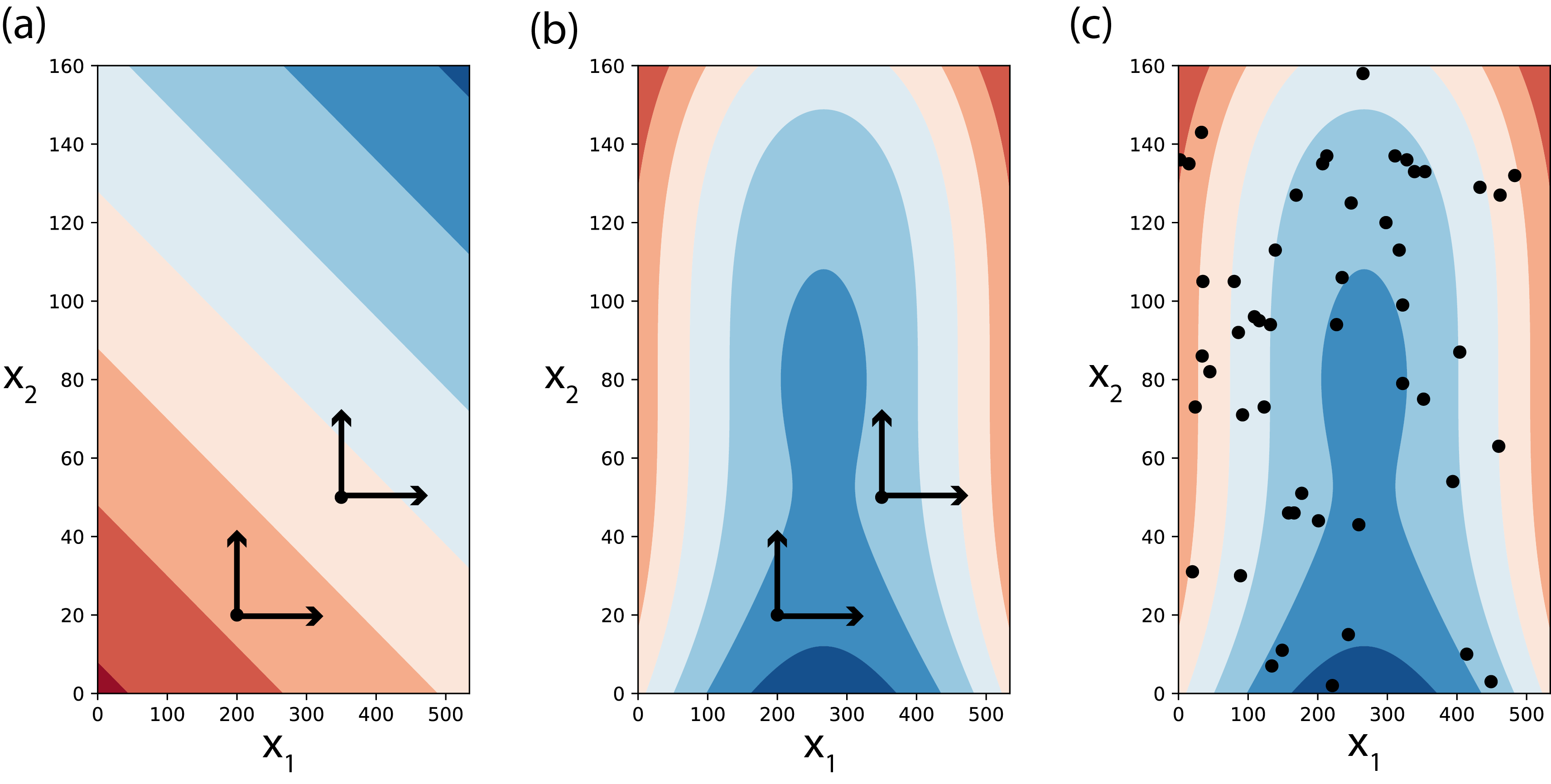
Comparison of Local vs. Global Sensitivity Analysis — This image provides a clear geometric intuition. The 'L' shaped arrows in plots (a) and (b) represent Local Sensitivity Analysis, where each variable (X1, X2) is perturbed independently from a base point. Plot (c) shows the Global approach, sampling across the entire space.

The image above visually demonstrates the OAT process. From a starting point, you move only along the X1 axis, then return to the start and move only along the X2 axis. The result is often visualized in a "Tornado Chart," which ranks the inputs by the magnitude of their impact.

Local Sensitivity Analysis Bar Chart — A typical output of a local OAT analysis. It shows the percentage change in an output resulting from a fixed percentage change (e.g., ±10%) in each input variable, ranked from most to least impactful.

Key Characteristics of LSA:

Methodology: Varies one input factor at a time (OAT), holding others fixed at a nominal "base case."
Scope: Explores the immediate vicinity of a single point in the parameter space.
Strength: Simple to implement and computationally cheap. It provides a rapid, first-order approximation of which variables are influential.
Critical Weakness: It assumes that the effect of changing one variable is independent of the values of the other variables. LSA cannot detect or quantify interactions between inputs. This is a significant drawback in non-linear systems, where the effect of one factor may be amplified or dampened by another. The sensitivity it calculates is only valid at the specific base case chosen.

Global Sensitivity Analysis (GSA): The Holistic View

Global Sensitivity Analysis overcomes the primary limitation of LSA. Instead of focusing on a single point, GSA evaluates the effect of an input while all other inputs are also varied over their entire range of uncertainty.

GSA does not rely on a single base case. Instead, it uses a sampling-based approach (often Monte Carlo methods) to explore the entire input space. It aims to apportion the variance of the model output to the variance of the input factors.

Global Sensitivity Analysis - Lecture Notes

This document from the SimCenter at UC Berkeley provides a concise and mathematically grounded distinction between local and global methods.

Read the section '6.1 Local versus Global' (pages 55-56). Focus on how it formally defines LSA as a partial derivative (OAT) and contrasts it with GSA, which 'considers the sensitivity across the ‘whole range’ of input space and considers also nonlinear dependencies.'

As the reading highlights, GSA can handle non-linear relationships and, most importantly, interactions. Looking back at the "Local vs. Global SA Methods" image, GSA corresponds to plot (c), where the model is evaluated at many points scattered across the entire feasible domain.

A popular GSA technique is Variance-Based SA, such as the Sobol method. This method decomposes the total variance of the output, $Var (Y)$ , into parts attributable to each input and their interactions. It calculates indices like:

First-Order Index ( $S_{i}$ ): The fraction of $Var (Y)$ caused by varying $X_{i}$ alone. This is the "main effect."
Total-Effect Index ( $S_{T i}$ ): The fraction of $Var (Y)$ caused by $X_{i}$ , including all its interactions with other inputs.

If $S_{T i}$ is much larger than $S_{i}$ for a given input, it's a strong indicator that this input is heavily involved in interactions with other factors.

Key Characteristics of GSA:

Methodology: Varies all input factors simultaneously, sampling from their probability distributions.
Scope: Explores the entire input parameter space.
Strength: Provides a robust and comprehensive understanding of sensitivities. It explicitly quantifies both main effects and interaction effects. The results are not dependent on a single "base case."
Critical Weakness: Computationally expensive. It may require thousands of model evaluations, which can be prohibitive for complex models.

Global Sensitivity Analysis

To solidify your understanding of the GSA mindset, this video explains why we need to think about input distributions and their effect on output distributions, moving beyond the local, derivative-based view.

Watch from 00:00 to 02:27 and from 03:03 to 06:19. The key concept here is framing the problem probabilistically: GSA relates the distribution of outputs to the distributions of inputs, allowing for more general and robust conclusions about the model's behavior.

Summary of Differences

The following table consolidates the core distinctions between local and global sensitivity analysis.

Feature	Local Sensitivity Analysis (e.g., OAT)	Global Sensitivity Analysis (e.g., Sobol)
Core Question	"What happens if I change one input, starting from this specific state?"	"How much does one input contribute to the output's total uncertainty, across all possible states?"
Input Variation	One at a time, around a fixed base case.	All at once, across their entire probability distributions.
Interaction Effects	Cannot be detected or quantified.	Can be explicitly quantified (e.g., via Total-Effect Indices).
Model Assumptions	Often implicitly assumes linearity or additivity.	Model-independent; handles non-linear and non-monotonic functions.
Computational Cost	Low (requires $2 k + 1$ or $k + 1$ model runs for $k$ inputs).	High (can require thousands of model runs).
Use Case	Rapid screening, identifying potentially important variables, simple models.	Robust model validation, understanding complex systems, policy support.

Conclusion

You now have a clear understanding of the fundamental divide in sensitivity analysis.

Local Sensitivity Analysis (LSA) is a myopic but fast approach. It's like standing in one spot and looking down each street one by one to see what's close by. Its OAT method is simple but blind to the complex interplay of factors in non-linear systems.
Global Sensitivity Analysis (GSA) is a panoramic, holistic approach. It's like having a satellite map of the entire city, showing how all the streets connect. It's computationally demanding but provides a far more robust and complete picture of the system's behavior, especially regarding interactions.

The choice is a classic trade-off between computational cost and analytical robustness.

Key Takeaways:

SA quantifies how input variations affect model output.
LSA (e.g., OAT) perturbs one input at a time from a single base case, making it fast but unable to capture interactions.
GSA (e.g., Sobol) varies all inputs simultaneously across their full ranges, making it robust and capable of quantifying interactions, but computationally expensive.

Preview of the Next Lesson:

While GSA is more robust, LSA is a pragmatic and powerful tool for an initial screening of your P_max model. It allows you to quickly identify the most likely candidates for your 'Hook' before committing to more complex analyses. In the next lesson, you will perform a one-at-a-time sensitivity analysis on a multi-variable model to rank the influence of each input on the output, taking the first practical step in quantitatively identifying your primary constraint.

Recommended resources