Counting Inversions with Merge Sort

1. What is an Inversion?

First, let's define the problem. An inversion in an array is a pair of indices (i, j) such that i < j but arr[i] > arr[j]. In simple terms, it's a pair of elements that are "out of order."

For example, in the array [3, 1, 2]:

• (3, 1) is an inversion because 3 > 1 and it appears before 1.
• (3, 2) is an inversion because 3 > 2 and it appears before 2.
• (1, 2) is not an inversion.

The total number of inversions is 2. The number of inversions is a measure of how "unsorted" an array is. A perfectly sorted array has 0 inversions, while a reverse-sorted array has the maximum possible number of inversions.

2. The Brute-Force Approach

As with many problems, the most straightforward solution is a good starting point. We can simply iterate through all possible pairs (i, j) where i < j and check if they form an inversion.

This involves a nested loop structure:

• An outer loop for the first element i.
• An inner loop for the second element j (starting from i + 1).

public static int countInversionsBruteForce(int[] arr) {
    int count = 0;
    for (int i = 0; i < arr.length - 1; i++) {
        for (int j = i + 1; j < arr.length; j++) {
            if (arr[i] > arr[j]) {
                count++;
            }
        }
    }
    return count;
}

This approach is correct, but its time complexity is O(n²), which is too slow for large arrays in an interview or competitive programming setting.

To see a quick walkthrough of the problem definition and this brute-force method, watch the first few minutes of the following video.

3. The Divide and Conquer Insight

To improve upon O(n²), we need a more clever approach. This is where your knowledge of Merge Sort comes in. Consider the "Divide and Conquer" structure:

Total Inversions = (Inversions in the left half) + (Inversions in the right half) + (Inversions between the two halves)

The first two components can be found by recursively calling our function on the left and right subarrays. The real challenge is counting the "cross-inversions"—pairs (arr[i], arr[j]) where arr[i] is in the left half, arr[j] is in the right half, and arr[i] > arr[j].

This is where the magic happens. The merge step of Merge Sort, where we combine two sorted subarrays, is the perfect place to count these cross-inversions efficiently.

Let's say we are merging two sorted subarrays, L and R. We use two pointers, i for L and j for R.

• If L[i] <= R[j], there's no inversion involving L[i] and R[j]. We just move L[i] to the merged array and advance i.
• If L[i] > R[j], we have found an inversion! But not just one. Since the left subarray L is sorted, we know that all remaining elements in L (from index i onwards) are also greater than or equal to L[i]. Therefore, they are all greater than R[j].

This means if L[i] > R[j], we have found (mid - i + 1) cross-inversions at once, where mid is the end of the left subarray.

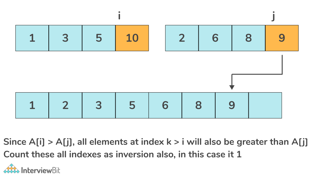
This single insight is what allows us to count inversions in O(n) time during the merge step, leading to an overall O(n log n) algorithm.

4. The Modified Merge Sort Algorithm

Now let's put it all together. The algorithm will look almost identical to Merge Sort, but our recursive function will now return an integer (the inversion count), and our merge function will also calculate and return the cross-inversion count.

The overall process is visualized well here:

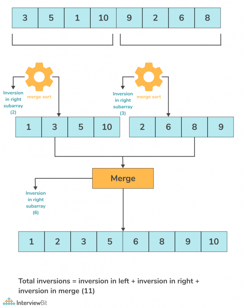
The full recursive logic is:

1. Base Case: If the array has 0 or 1 element, return 0 inversions.
2. Divide: Split the array into two halves.
3. Conquer: Recursively call the function on both halves. Sum their returned inversion counts: count = countInversions(left) + countInversions(right).
4. Combine: Merge the two sorted halves back together. During the merge, count the cross-inversions and add them to your total: count += mergeAndCount(left, right).
5. Return the total count.

5. Java Implementation

Let's look at a clean implementation. The structure will have a main recursive function, mergeSortAndCount, and a helper function, mergeAndCount.

Here is a consolidated version of the code, based on the Baeldung article, for your reference.

import java.util.Arrays;

public class InversionCounter {

    // Main recursive function to sort and count inversions
    private static long mergeSortAndCount(int[] arr, int left, int right) {
        long inversionCount = 0;
        if (left < right) {
            int mid = left + (right - left) / 2;

            // Count inversions in left subarray
            inversionCount += mergeSortAndCount(arr, left, mid);

            // Count inversions in right subarray
            inversionCount += mergeSortAndCount(arr, mid + 1, right);

            // Count cross-inversions during merge
            inversionCount += mergeAndCount(arr, left, mid, right);
        }
        return inversionCount;
    }

    // Function to merge two sorted halves and count cross-inversions
    private static long mergeAndCount(int[] arr, int left, int mid, int right) {
        // Create temporary arrays for left and right halves
        int[] leftSub = Arrays.copyOfRange(arr, left, mid + 1);
        int[] rightSub = Arrays.copyOfRange(arr, mid + 1, right + 1);

        int i = 0; // Pointer for leftSub
        int j = 0; // Pointer for rightSub
        int k = left; // Pointer for the original array
        long crossInversions = 0;

        while (i < leftSub.length && j < rightSub.length) {
            if (leftSub[i] <= rightSub[j]) {
                arr[k++] = leftSub[i++];
            } else {
                arr[k++] = rightSub[j++];
                // This is the key step!
                crossInversions += (leftSub.length - i);
            }
        }

        // Copy remaining elements of leftSub (if any)
        while (i < leftSub.length) {
            arr[k++] = leftSub[i++];
        }

        // Copy remaining elements of rightSub (if any)
        while (j < rightSub.length) {
            arr[k++] = rightSub[j++];
        }

        return crossInversions;
    }

    public static long countInversions(int[] arr) {
        if (arr == null || arr.length < 2) {
            return 0;
        }
        // Create a copy to avoid modifying the original array, which is good practice.
        int[] arrCopy = Arrays.copyOf(arr, arr.length);
        return mergeSortAndCount(arrCopy, 0, arrCopy.length - 1);
    }

    public static void main(String[] args) {
        int[] arr = {8, 4, 2, 1};
        System.out.println("Number of inversions are: " + countInversions(arr)); // Output: 6
    }
}

6. Complexity Analysis

• Time Complexity: We added a single line of code that does a constant-time arithmetic operation inside the merge function. The overall structure of the algorithm remains identical to Merge Sort. Therefore, the time complexity is still O(n log n).
• Space Complexity: We are still using a temporary array (or two) of size proportional to n for the merging process. Therefore, the auxiliary space complexity is O(n).

This is a massive improvement over the O(n²) brute-force solution and is efficient enough to pass in any interview or competitive programming context.

Conclusion

Great job! You've just learned how to solve a non-trivial problem by adapting a fundamental algorithm. This demonstrates a deeper level of understanding than simply memorizing sorting algorithms.

Key Takeaways:

• An inversion is a pair of elements (arr[i], arr[j]) where i < j and arr[i] > arr[j].
• A brute-force O(n²) solution exists but is inefficient.
• The Divide and Conquer strategy of Merge Sort can be used to count inversions efficiently.
• The key insight is to count cross-inversions during the merge step. When leftSub[i] > rightSub[j], all remaining elements in the sorted leftSub also form an inversion with rightSub[j].
• The final algorithm runs in O(n log n) time and uses O(n) space, just like Merge Sort.

Preview of the next lesson:
We have now thoroughly covered Merge Sort and one of its powerful applications. Next, we will explore another famous O(n log n) sorting algorithm: Quick Sort. It also uses a "Divide and Conquer" approach but employs a different strategy called "partitioning." We will implement it, analyze its performance—which has different best/worst-case characteristics than Merge Sort—and discuss when you might choose one over the other.