Quick Sort: Lomuto, Hoare, and Performance Analysis

1. The Core Idea: Partitioning

While Merge Sort blindly splits the array in half, Quick Sort intelligently divides it. The core operation is partition(), which takes an array (or subarray) and does the following:

1. Selects an element called the "pivot".
2. Rearranges the array so that all elements smaller than the pivot come before it, and all elements greater than the pivot come after it.
3. After partitioning, the pivot is in its final, sorted position.

This process creates two smaller subarrays that can then be sorted recursively.

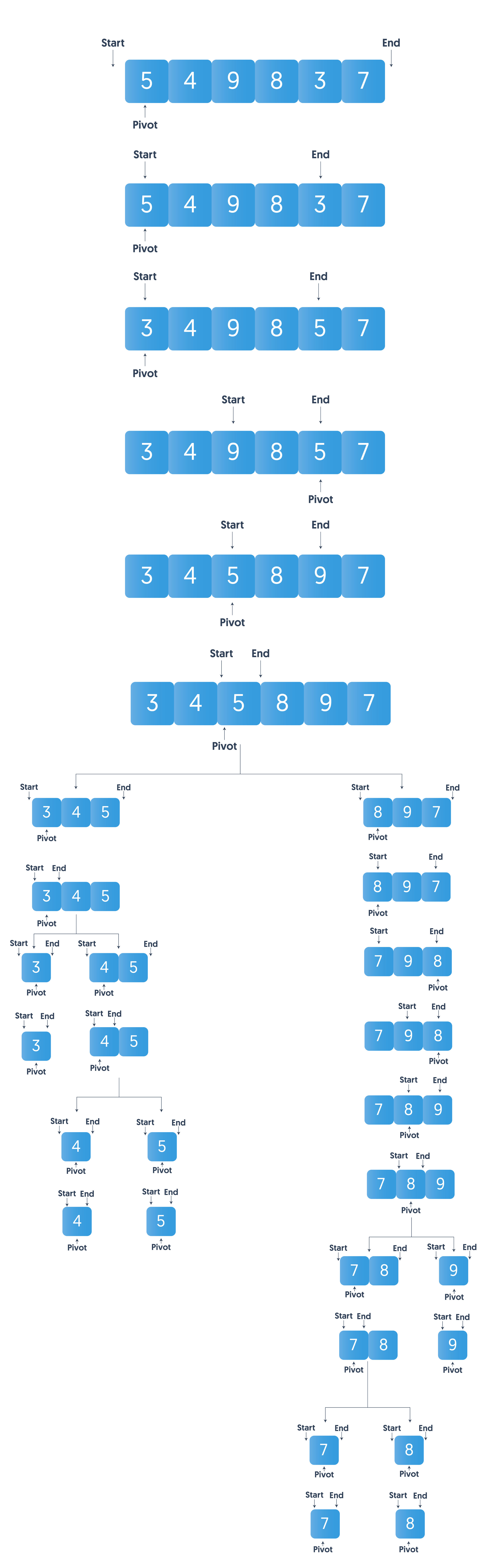
This diagram illustrates the Quick Sort process. First, the array is partitioned around a pivot (5), placing smaller elements to the left and larger ones to the right. Then, the algorithm recursively sorts the left and right subarrays.

To get a solid high-level understanding of this concept before we dive into code, let's consult a well-written overview.

Now that you have the general idea, let's implement it. There are two famous ways to perform the partition step. We'll start with the more intuitive one.

2. The Lomuto Partition Scheme

The Lomuto scheme is popular because it's easier to grasp and implement correctly. It generally works as follows:

• The pivot is chosen as the last element of the array.
• A pointer, i, is initialized just before the start of the array (low - 1). This i will mark the boundary between elements less than or equal to the pivot and those greater than it.
• Another pointer, j, iterates from the start of the array (low) up to the element just before the pivot.
• If arr[j] is less than or equal to the pivot, we increment i and then swap arr[i] with arr[j]. This effectively expands the region of "smaller" elements by one and places arr[j] within it.
• After the loop finishes, all elements from low to i are less than or equal to the pivot. The final step is to swap the pivot (originally at arr[high]) with arr[i + 1], placing it in its correct sorted position. The function then returns this position i + 1.

Let's look at a standard implementation.

Here is a complete Java implementation for Quick Sort using Lomuto's partition.

public class QuickSortLomuto {

    // Main function that implements QuickSort
    public static void quickSort(int[] arr, int low, int high) {
        if (low < high) {
            // pi is the partitioning index, arr[pi] is now at its right place
            int pi = partition(arr, low, high);

            // Recursively sort elements before and after the partition
            quickSort(arr, low, pi - 1);
            quickSort(arr, pi + 1, high);
        }
    }

    // This function takes the last element as pivot, places the pivot element
    // at its correct position in the sorted array, and places all smaller
    // elements to the left of the pivot and all greater elements to the right.
    static int partition(int[] arr, int low, int high) {
        int pivot = arr[high];
        int i = (low - 1); // Index of smaller element

        for (int j = low; j < high; j++) {
            // If the current element is smaller than or equal to the pivot
            if (arr[j] <= pivot) {
                i++;
                // Swap arr[i] and arr[j]
                int temp = arr[i];
                arr[i] = arr[j];
                arr[j] = temp;
            }
        }

        // Swap the pivot element with the element at i + 1
        int temp = arr[i + 1];
        arr[i + 1] = arr[high];
        arr[high] = temp;

        return (i + 1);
    }
}

3. The Hoare Partition Scheme

The Hoare scheme is the original partition method published by Tony Hoare. It's slightly more complex but generally more efficient as it performs fewer swaps on average.

• The pivot is typically chosen as the first element.
• It uses two pointers, i starting just before the first element and j just after the last element.
• The pointers move towards each other: i moves right, skipping over elements smaller than the pivot, and j moves left, skipping over elements greater than the pivot.
• When both pointers stop, i is at an element arr[i] >= pivot and j is at an element arr[j] <= pivot.
• If i < j, it means we've found an "inversion" (a large element on the left and a small one on the right), so arr[i] and arr[j] are swapped.
• This process repeats until the pointers i and j cross or meet (i >= j). The function then returns j.

Crucial Point: Unlike Lomuto's scheme, Hoare's scheme does not necessarily place the pivot at its final sorted position. It only guarantees that it returns a split index j such that all elements to the left of j are less than or equal to the pivot, and all elements to the right of j are greater than or equal to the pivot. This changes how we make the recursive calls.

Here is the corresponding Java code for Quick Sort using Hoare's partition.

public class QuickSortHoare {

    public static void quickSort(int[] arr, int low, int high) {
        if (low < high) {
            int pi = partition(arr, low, high);

            // Recursively sort elements before and after the partition index.
            // Note the `pi` in the first call, not `pi - 1`.
            quickSort(arr, low, pi);
            quickSort(arr, pi + 1, high);
        }
    }

    // This function partitions the array using the first element as the pivot.
    // It returns an index j such that all elements to the left are <= pivot
    // and all elements to the right are >= pivot.
    static int partition(int[] arr, int low, int high) {
        int pivot = arr[low];
        int i = low - 1;
        int j = high + 1;

        while (true) {
            // Find an element on the left side that is not smaller than the pivot
            do {
                i++;
            } while (arr[i] < pivot);

            // Find an element on the right side that is not greater than the pivot
            do {
                j--;
            } while (arr[j] > pivot);

            // If pointers have crossed, the partition is done
            if (i >= j) {
                return j;
            }

            // Swap arr[i] and arr[j]
            int temp = arr[i];
            arr[i] = arr[j];
            arr[j] = temp;
        }
    }
}

4. Performance Analysis

Quick Sort's performance is heavily dependent on the quality of the pivots chosen.

Time Complexity

• Best Case: O(n log n)
  This occurs when the partition step always divides the array into two nearly equal halves. Each level of recursion processes n elements, and there are log n levels.

*This slide illustrates the best-case scenario for Quick Sort. The work at each level of the recursion tree is O(n), and the height of the tree is O(log n), leading to an overall time complexity of O(n log n).*

• Average Case: O(n log n)
  Even with slight imbalances in partitions, Quick Sort maintains its efficiency. It has been mathematically proven to be very fast on average for random inputs.

• Worst Case: O(n²)
  This is the most important case to understand for interviews. It occurs when the partition step consistently produces highly unbalanced splits (e.g., one subarray of size 0 and another of size n-1). This happens on an already sorted or reverse-sorted array if you naively pick the first or last element as the pivot. The recursion depth becomes n, leading to n * n = n² comparisons.

Space Complexity

• Average Case: O(log n)
  This is due to the recursion stack depth. Since the partitions are balanced, the call stack only goes log n levels deep. This is a significant advantage over Merge Sort's O(n) space complexity.
• Worst Case: O(n)
  In the worst-case scenario of unbalanced partitions, the recursion depth can become n, leading to O(n) space complexity for the call stack.

Mitigating the Worst Case

Because the O(n²) worst case is so detrimental, in practice, you should never naively pick the first or last element. Common strategies to avoid this include:

1. Randomized Pivot: Pick a random element as the pivot. This makes it extremely unlikely for the worst-case to occur on any given input.
2. Median-of-Three: Take the first, middle, and last elements of the subarray, and choose their median as the pivot. This is a good heuristic that avoids the pitfalls of sorted arrays.

Conclusion

Excellent work! You've now implemented and analyzed one of the most widely used and fastest known sorting algorithms. Understanding the nuances between its different partitioning schemes and its performance characteristics is a hallmark of a strong software engineer.

Key Takeaways:

• Quick Sort is an in-place, "Divide and Conquer" sorting algorithm. Its primary operation is partitioning.
• Lomuto's scheme is simpler to implement, uses the last element as a pivot, and places the pivot in its final correct position.
• Hoare's scheme is the original, generally performs fewer swaps, but is slightly more complex. It returns a split point, and the pivot itself is not necessarily in its final position after one partition.
• Quick Sort's average time complexity is a very fast O(n log n) with an average space complexity of O(log n).
• Its worst-case time complexity is O(n²), which can be mitigated by using a smart pivot selection strategy like randomization or median-of-three.

Preview of the next lesson:
We have now covered several "comparison-based" sorting algorithms (Merge Sort, Quick Sort). Their theoretical best-case time complexity is O(n log n). But what if we could sort without comparing elements? In the next lesson, we will explore Counting Sort, a linear-time sorting algorithm that works under specific constraints on the input data.