Merge Sort: Implementation and Complexity Analysis

1. The "Divide and Conquer" Strategy

Merge Sort breaks down a large, difficult problem (sorting an entire array) into smaller, easier-to-solve subproblems, and then combines their solutions to solve the original problem.

It operates in two main phases:

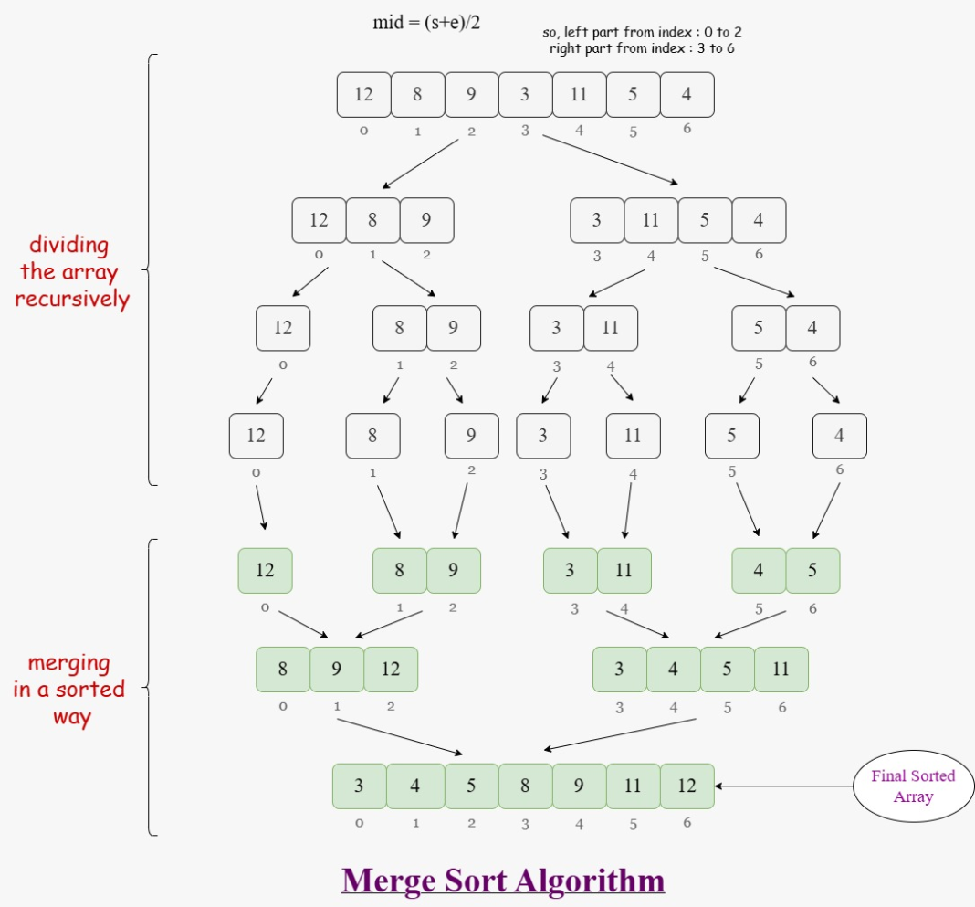
1. Divide: Recursively split the array in half until you are left with arrays containing just one element. A single-element array is, by definition, already sorted. This is our recursive base case.
2. Conquer (Merge): Take the sorted single-element arrays and start merging them back together. You merge two sorted arrays of size 1 to get a sorted array of size 2. Then you merge two sorted arrays of size 2 to get a sorted array of size 4, and so on, until you have one final, completely sorted array.

This diagram provides a perfect visual summary of the process:

To get a feel for this process, let's watch a brief conceptual overview.

2. Implementation in Java

Now, let's translate this "divide and conquer" logic into Java code. We'll build two main methods:

• mergeSort(): A recursive method that handles the "divide" part.
• merge(): A helper method that handles the "conquer" part, merging two sorted subarrays.

We'll follow the implementation from the same video. It's a clear, well-explained walkthrough that's perfect for your practical learning style.

The mergeSort() (Divide) Method

The mergeSort method is the recursive driver. Its job is to:

1. Check for the base case: if the array has fewer than two elements, it's already sorted, so we just return.
2. Find the middle index of the array.
3. Create two new temporary arrays: leftHalf and rightHalf.
4. Copy the corresponding elements from the input array into these two halves.
5. Recursively call mergeSort() on the leftHalf.
6. Recursively call mergeSort() on the rightHalf.
7. Call the merge() method to combine the now-sorted leftHalf and rightHalf back into the original array.

The merge() (Conquer) Method

This is the heart of the algorithm where the actual sorting happens. The merge method takes two already sorted arrays and combines them into one larger sorted array. The logic uses the two-pointer technique:

1. Create three pointers: i for the left half, j for the right half, and k for the main array we're filling.
2. While there are still elements in both halves:
   • Compare the elements at leftHalf[i] and rightHalf[j].
   • Copy the smaller of the two into the main array at a[k].
   • Increment the pointer of the half you took the element from (i or j), and always increment the main array's pointer (k).
3. Once one of the halves is exhausted, copy all remaining elements from the other half into the main array.

Here is the complete Java code for your reference, which matches the implementation in the video.

public class MergeSort {

    public static void mergeSort(int[] inputArray) {
        int inputLength = inputArray.length;

        // Base case: An array with 0 or 1 element is already sorted.
        if (inputLength < 2) {
            return;
        }

        // 1. Divide
        int midIndex = inputLength / 2;
        int[] leftHalf = new int[midIndex];
        int[] rightHalf = new int[n - midIndex];

        // Populate the left and right halves
        for (int i = 0; i < midIndex; i++) {
            leftHalf[i] = inputArray[i];
        }
        for (int i = midIndex; i < inputLength; i++) {
            rightHalf[i - midIndex] = inputArray[i];
        }

        // Recursively sort each half
        mergeSort(leftHalf);
        mergeSort(rightHalf);

        // 2. Conquer (Merge)
        merge(inputArray, leftHalf, rightHalf);
    }

    private static void merge(int[] inputArray, int[] leftHalf, int[] rightHalf) {
        int leftSize = leftHalf.length;
        int rightSize = rightHalf.length;

        int i = 0; // Pointer for the left half
        int j = 0; // Pointer for the right half
        int k = 0; // Pointer for the main input array

        // Compare elements and merge
        while (i < leftSize && j < rightSize) {
            if (leftHalf[i] <= rightHalf[j]) {
                inputArray[k] = leftHalf[i];
                i++;
            } else {
                inputArray[k] = rightHalf[j];
                j++;
            }
            k++;
        }

        // Clean up remaining elements
        while (i < leftSize) {
            inputArray[k] = leftHalf[i];
            i++;
            k++;
        }
        while (j < rightSize) {
            inputArray[k] = rightHalf[j];
            j++;
            k++;
        }
    }
}

3. Complexity Analysis

Analyzing Merge Sort is a classic interview topic. Its efficiency comes from its O(n log n) time complexity. Let's break down where the n and log n come from.

Time Complexity: O(n log n)

The complexity can be understood by looking at the two parts of the algorithm's name:

• log n (from "Sort"): This comes from the dividing phase. How many times can you split an array of size n in half before you get down to arrays of size 1? The answer is log₂(n). This determines the number of levels in our recursion.
• n (from "Merge"): This comes from the merging phase. At each of the log n levels of recursion, we perform a series of merge operations. If you sum the sizes of all subarrays at any given level, it will always equal n. Since the merge operation takes linear time proportional to the number of elements it's merging, the total work done at each level is O(n).

So, we have log n levels, and at each level, we do O(n) work. This gives us a total time complexity of O(n log n).

One of the most important properties of Merge Sort is that this complexity is consistent. It's O(n log n) for the best, average, and worst cases because the array is always split in half, and the merge process always visits every element, regardless of the input's initial order.

Space Complexity: O(n)

Merge Sort's primary weakness is its space complexity.

• Auxiliary Space: In the implementation we've used (which is standard), we create temporary leftHalf and rightHalf arrays at each level of recursion. The maximum space required for these temporary arrays at any one time is when we are merging the two largest halves, each of size approximately n/2, which requires O(n) auxiliary space.
• Recursion Stack Space: The recursive calls also consume space on the call stack. The depth of the recursion tree is O(log n), so this adds O(log n) space.

The auxiliary space O(n) dominates the recursion stack space O(log n). Therefore, the overall space complexity is O(n). This is a crucial trade-off: Merge Sort gains speed but at the cost of using extra memory. This is why it's not an "in-place" algorithm like the O(n²) sorts we studied previously.

Conclusion

Congratulations on tackling your first O(n log n) sorting algorithm! Merge Sort is a cornerstone of efficient sorting and a beautiful example of recursive problem-solving.

Key Takeaways:

• Merge Sort uses a Divide and Conquer strategy to achieve a time complexity of O(n log n).
• This time complexity is consistent across best, average, and worst-case scenarios.
• The merge step, which combines two sorted subarrays in linear time, is the core of the algorithm.
• Its main disadvantage is its O(n) space complexity, as it requires temporary arrays for merging.
• Merge Sort is a stable sort, meaning it preserves the relative order of equal elements.

Preview of the next lesson:
The real power of Merge Sort extends beyond just sorting. The merge function is a versatile pattern. In our next lesson, we will see how a slight modification to this function allows us to solve a completely different problem: counting inversions in an array. This is a classic, challenging problem that frequently appears in competitive programming and advanced interviews, and it builds directly on the foundation you've built today.