Decoupled Fixed-Timestep Simulation

The Problem with a Naive Game Loop

As we discussed, a simple game loop ties the simulation step directly to the rendering frame rate. This is problematic. A powerful computer might run at 500 frames per second, while a slower one might manage only 30. If an object's velocity is updated each frame, its speed in the game world becomes dependent on the player's hardware.

A common first attempt to fix this is to measure the time elapsed since the last frame (the "delta time" or dt) and scale all movement by that value. While this makes the game's speed consistent, it introduces a more subtle and dangerous problem for physics.

To see a clear visual explanation of this dilemma, let's watch the first part of a helpful video.

The video highlights two critical issues for a physics engine:

1. Instability: Numerical integrators, which we will use to solve the equations of motion, are tuned for a specific time step. A large, unpredictable dt can cause them to "blow up," leading to objects flying off to infinity.
2. Non-Determinism: Floating-point arithmetic rounding errors accumulate differently depending on the number and size of the steps. With a variable dt, the same initial conditions and inputs can produce different results on different machines, making debugging and networked multiplayer nearly impossible.

For a more in-depth analysis of these problems, we'll turn to a classic article on the topic.

The Accumulator Pattern: Decoupling Simulation and Rendering

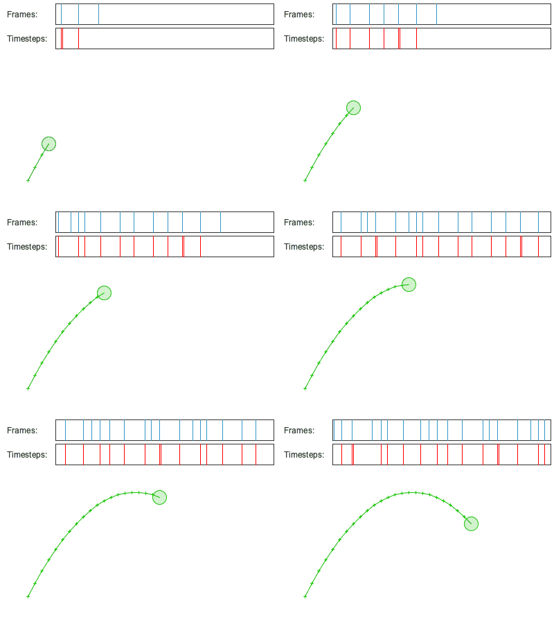
The solution is to "free the physics" from the rendering loop. We will run our simulation with a constant, small time step (e.g., dt = 1/60 of a second), but we'll do it in a way that keeps pace with real-world time.

The core idea is to treat time as a resource. The rendering loop produces an amount of real-world time each frame. The physics simulation consumes that time in fixed, discrete chunks. Any unconsumed time is saved for the next frame. This is managed with a variable often called an accumulator.

The logic is as follows:

1. Measure the real time that has passed since the last frame (frameTime).
2. Add this frameTime to an accumulator.
3. While the accumulator is greater than our fixed physics dt, perform one physics step and subtract dt from the accumulator.
4. Repeat until the accumulator is less than dt.
5. Render the scene.

This ensures the physics simulation is always updated with the same dt, providing stability and determinism, while also allowing the simulation to "catch up" if the rendering frame rate drops by executing multiple physics steps in a single frame.

Let's read about this elegant solution in more detail.

The "Game Programming Patterns" book offers another excellent perspective on this same pattern, which may help solidify your understanding.

Implementing the Loop in C++

Now, let's translate this pseudocode into a working C++ structure. You'll need a main loop that will eventually house your engine.

1. Measuring Time
First, we need a way to accurately measure frameTime. The C++ <chrono> library is perfect for this, providing high-resolution, cross-platform clocks.

A practical tutorial video demonstrates how to set up a function for this and structure the main loop.

Your basic loop structure in C++ will look something like this. You can now start building this out in your project.

#include <chrono>

// High-resolution clock
using Clock = std::chrono::high_resolution_clock;
using TimePoint = std::chrono::time_point<Clock>;

int main() {
    const double dt = 1.0 / 60.0; // Physics timestep
    double accumulator = 0.0;

    TimePoint currentTime = Clock::now();

    bool running = true;
    while (running) {
        TimePoint newTime = Clock::now();
        double frameTime = std::chrono::duration<double>(newTime - currentTime).count();
        currentTime = newTime;

        // Defensive clamp for when debugging, pausing, or moving the window
        if (frameTime > 0.25) {
            frameTime = 0.25;
        }

        accumulator += frameTime;

        while (accumulator >= dt) {
            // previousState = currentState; // We'll need this for interpolation
            // integrate(currentState, dt);
            accumulator -= dt;
        }

        // render(currentState, accumulator / dt);
    }

    return 0;
}

The Final Touch: Smoothing with Interpolation

There's one final problem to solve. Our physics state (currentState) only updates in discrete dt intervals. However, the render() function is called at arbitrary times between those updates. This means the rendered object will appear to "jump" from one position to the next every dt seconds, causing a visual stutter, especially if the render rate is much higher than the physics rate.

The value left in the accumulator after the physics while loop finishes tells us exactly how far we are into the next physics step, timewise. For example, if accumulator is 0.5 * dt, we are halfway to the next physics update. We can use this fraction, often called alpha, to interpolate between the object's state at the last physics step (previousState) and its state at the current one (currentState).

alpha = accumulator / dt;

The rendered position would then be:
renderPosition = currentState.position * alpha + previousState.position * (1.0 - alpha);

This gives the illusion of perfectly smooth motion, even though the underlying physics simulation is ticking along at a coarser, fixed rate. Your OpenGL experience will be useful here, as this interpolated state is what you will ultimately pass to your rendering pipeline.

Let's conclude our reading to see how this is formally described.

Conclusion

In this lesson, we have moved beyond theory to construct the fundamental loop that will power our physics engine. This is a critical piece of infrastructure that ensures your simulation will be stable, predictable, and behave consistently across all hardware.

Here are the key takeaways:

• Tying simulation to rendering frame rate or using a variable time step leads to instability and non-deterministic behavior in a physics simulation.
• The solution is to decouple the loops, using a fixed time step (dt) for physics updates.
• The accumulator pattern allows the fixed-step simulation to keep pace with real-world time, running multiple updates per frame if necessary.
• To avoid visual stutter, the rendered state should be interpolated between the previous and current physics states using the remainder in the accumulator as the blending factor.

You now have the core loop of an engine. In the next lesson, we will put this structure to use and satisfy your preference for visual feedback by setting up a basic debug drawing system using OpenGL. This will allow us to see the results of our future work, starting with vectors, matrices, and particle motion.