Hello! Welcome to the fourth lesson in our journey into Bayesian thinking.
In our last session, we dissected Bayes' theorem and gave each of its components—prior, likelihood, posterior, and evidence—a clear, conceptual meaning using the medical diagnosis problem. We ended with a question: what happens when we get more evidence, like a second positive test?
Today, we'll answer that question directly. We are going to explore one of the most powerful and elegant features of the Bayesian framework: its iterative nature. You will learn how Bayesian analysis is not a static, one-time calculation but a dynamic process of learning, where the conclusion from one step becomes the starting point for the next. This formalizes the very natural human process of updating our understanding as we gather more information.
1. From Posterior to Prior: Revisiting the Medical Diagnosis
Let's pick up exactly where we left off. In the Veritasium video, after a single positive test for a rare disease (with a 0.1% prevalence), the probability of actually having the disease—our posterior—was found to be only about 9%.
So, what happens if you get a second opinion from an independent lab, and that test also comes back positive? Does the probability stay at 9%? Intuitively, we know our belief should get stronger. But by how much?
The key insight is this: our state of knowledge has changed. We are no longer a random person from the general population. We are now a person with one piece of incriminating evidence. Therefore, our new prior probability is no longer the base rate of 0.1%, but the 9% posterior we just calculated.
The following clip from "The Bayesian Trap" demonstrates this update in action.
Watch this segment from 'The Bayesian Trap' to see how the posterior from the first test becomes the prior for the second test.
Watch from 05:05 to 05:57. Notice how the calculation is repeated, but this time the prior probability P(Hypothesis) is set to 0.09 (or 9%), our result from the first analysis.
As the video shows, by incorporating the second positive test, our belief jumps dramatically from 9% to 91%. This is the core mechanism of Bayesian learning:
Posterior from round 1 → Prior for round 2
This cycle of updating our beliefs as evidence arrives is a fundamental concept.
2. The Bayesian Learning Cycle
This iterative process can be visualized as a continuous loop. It's a formal model for how we, as humans, learn from experience.
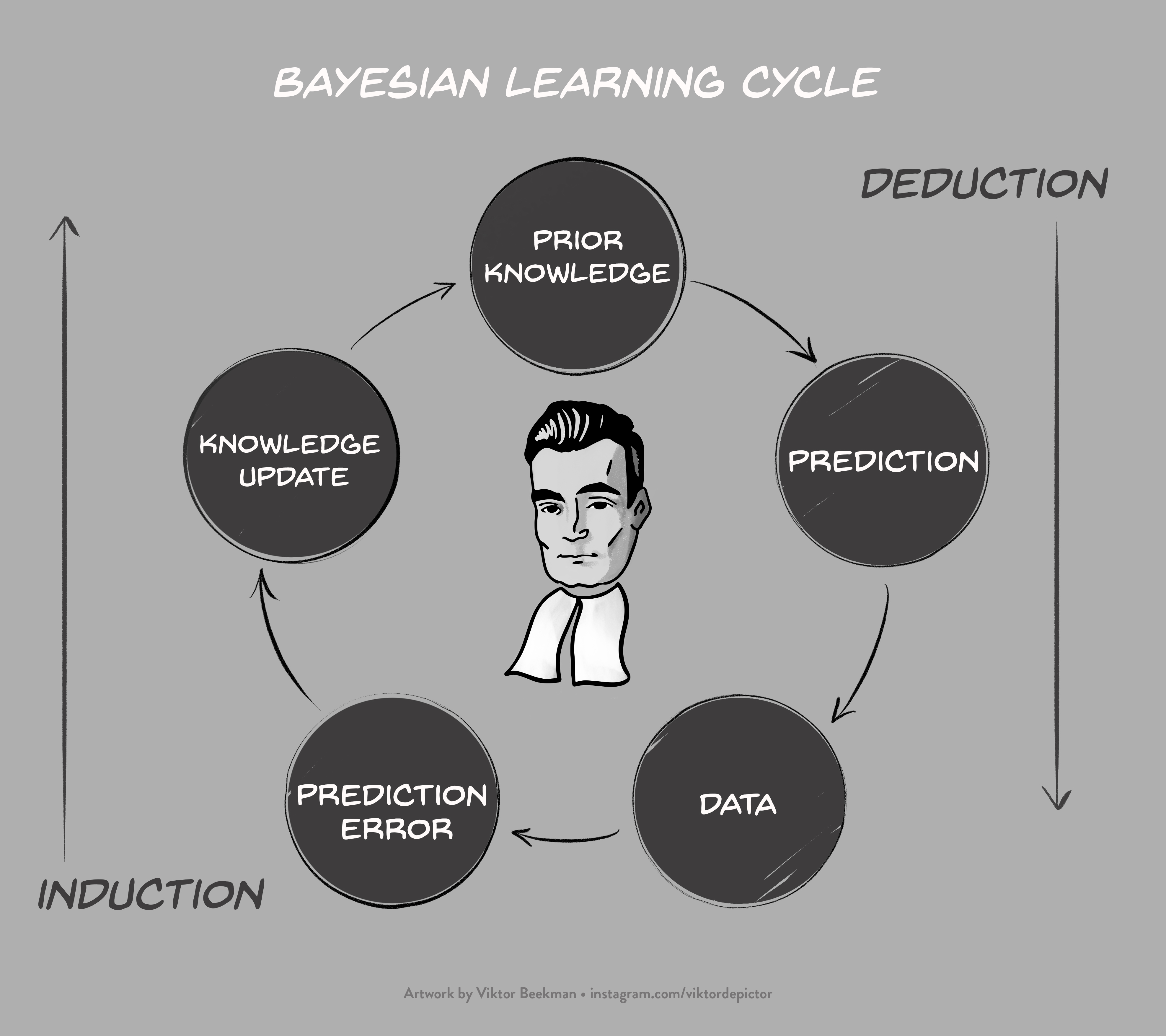
This cycle—sometimes called the "Bayesian Learning Cycle"—is what allows an analyst or a machine learning model to refine its "worldview" with every new data point it observes.
3. A Step-by-Step Example: Detecting a Biased Coin
Let's move from the high-level concept to the nuts and bolts. We'll work through a classic problem: trying to determine if a coin is fair or biased based on a sequence of flips. This will give you a concrete feel for the math behind sequential updates.
The following text provides a clear, step-by-step walkthrough of this exact problem.
4.5. Sequential Bayesian Updating — STAT 350
The following resource, 'Sequential Bayesian Updating', details how to update your belief about a coin being biased after each successive flip results in heads.
Please read from the beginning of the section '4.5.1. Detecting a Biased Coin' down to the end of the 'Flip 3' subsection. As you read, focus on: The initial setup: What is the prior probability of having the biased coin? The calculation for 'Flip 1': How does the first 'Heads' update the probability? The calculation for 'Flip 2': Notice how the posterior from Flip 1 (≈0.151) is explicitly used as the new prior for this second step.
As you saw in the reading, the process is methodical:
- Start with a prior:
- Observe data (Flip 1 is Heads): Calculate the posterior, .
- Prepare for the next update: This posterior becomes our new prior.
- Observe more data (Flip 2 is Heads): Use the new prior of 0.151 to calculate the next posterior, .
- ...and so on.
The summary table in the resource shows this evolution beautifully. After 10 consecutive heads, the belief that the coin is biased climbs from a mere 10% to over 92%. The evidence gradually overwhelms our initial (low) prior belief.
4. Yesterday's Posterior is Today's Prior
This idea of sequential updating is not just a mathematical curiosity; it mirrors how we reason about the world. When you're debugging code, you don't throw away your conclusions from the last test you ran. Instead, the result of that test informs what you try next. Bayesian inference is the formal language for this process.
The following video provides a couple of great analogies to help cement this idea.
You Know I'm All About that Bayes: Crash Course Statistics #24
This clip from Crash Course Statistics uses a fun example about a blind date to illustrate sequential updating and concludes with a very memorable phrase.
Watch from 02:54 to 05:38, focusing on the story of Maria and Jordan. Notice how her belief is updated first by one piece of evidence (he saw the movie) and then can be updated again by a second (his dog's name). Then, watch the short concluding clip from 11:04 to 11:24 for the key takeaway.
As the host succinctly puts it: "Yesterday's posterior is today's prior." This is perhaps the most famous summary of Bayesian learning.
Test your understanding!
Let's return to the biased coin example from the reading. After 10 consecutive heads, the posterior probability of having the biased coin was .
Now, imagine the 11th flip is Tails.
Given:
- The probability of tails for the biased coin is .
- The probability of tails for a fair coin is .
Using as your new prior, calculate the updated posterior probability . Does the evidence of a single tail significantly change your strong belief?
Show answer
We apply Bayes' theorem one more time. Our prior is , so . Our new evidence is "Tails" (T).
The probability dropped from ~92% to ~83%. A single tail, which is more likely with a fair coin than the biased one, provided significant evidence against the "biased" hypothesis and noticeably weakened our belief, even after 10 confirming heads.
Conclusion
In this lesson, we've unlocked a core feature of Bayesian statistics: its capacity for sequential learning.
Key Takeaways:
- Bayesian inference is an iterative process, not a one-off calculation.
- The posterior probability from one stage of analysis becomes the prior probability for the next stage.
- This mechanism allows us to update our beliefs incrementally as new evidence becomes available.
- This process, summarized as "yesterday's posterior is today's prior," is a formal version of how we naturally learn from accumulating experience.
Next time:
So far, we've focused on updating our belief about one or two competing hypotheses (e.g., disease vs. no disease). But Bayesian analysis is a framework for achieving several different kinds of goals. In our next lesson, we will step back and distinguish between the three primary tasks you can accomplish with a Bayesian model: estimation, hypothesis testing, and prediction. This will give us a roadmap for the practical applications we'll explore in the rest of the course.