Unpacking Bayes' Theorem: A Medical Diagnosis Example

1. The Bayesian Trap: When Intuition Fails

Let's start with a scenario. You take a medical test for a rare disease. The test is highly accurate, and your result is positive. What is the probability that you actually have the disease? Most people's intuition gets this spectacularly wrong.

The following video from Veritasium sets up this exact problem. It highlights the common logical pitfall and introduces Bayes' theorem as the tool to get us out of it.

The common, intuitive answer is to say the probability is 99%, the same as the test's accuracy. As the video states, this is incorrect. The actual probability is much, much lower. This startling gap between our intuition and the mathematical reality is why a formal framework is so essential. Let's unpack why this happens.

2. Thinking with Frequencies: An Intuitive Solution

Your preference for starting with simple, intuitive explanations is perfect for this problem. The confusion arises from working with percentages and conditional probabilities directly. A much clearer way to think about it, especially at first, is to use "natural frequencies"—that is, imagining a concrete number of people and tracking them through the process.

This approach bypasses the confusing formulas and makes the logic transparent. You've worked with large datasets as a machine learning engineer, so thinking in terms of population counts should feel natural.

As the video demonstrates, the key is to realize that while the test is accurate, the disease is very rare. Out of a large population, the small percentage of "false positives" from the huge group of healthy people ends up being a larger absolute number than the "true positives" from the tiny group of sick people.

When you test positive, you don't know which group you're in. The probability is therefore the ratio of true positives to the total number of positive tests (true positives + false positives). This is the core insight that Bayes' theorem formalizes.

3. Naming the Parts: The Language of Bayes' Theorem

Now that we have the intuition, let's map it onto the formal structure of Bayes' theorem. Let $H$ stand for our Hypothesis ("the patient has the disease") and $D$ stand for our Data ("the test was positive").

Bayes' theorem is a statement about how our belief in the hypothesis should change after observing the data.

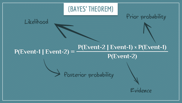
Let's define each part using the medical diagnosis example:

1. Prior Probability: $P(H)$

• What it is: The probability of the hypothesis before we see the data. It's our initial degree of belief.
• In our example: This is the base rate, or prevalence, of the disease. In the Veritasium example, $P(\text{Disease})=0.001$. This is our starting point. It reflects the fact that, without any other information, we'd assume any random person has a very low chance of having this rare disease.

2. Likelihood: $P(D|H)$

• What it is: The probability of observing the data given that our hypothesis is true. This term connects the data to the hypothesis. It answers the question: "How likely would I be to see this evidence if my theory were correct?"
• In our example: This is the test's sensitivity or true positive rate. $P(\text{Positive Test}|\text{Disease})=0.99$. It tells us how well our hypothesis (the patient has the disease) explains the data (a positive test). Note that this is not the probability of the hypothesis!

3. Posterior Probability: $P(H|D)$

• What it is: The probability of the hypothesis after we have taken the data into account. This is the updated belief and the quantity we usually want to find.
• In our example: This is $P(\text{Disease}|\text{Positive Test})$, the probability a person actually has the disease given they tested positive. This was the 9% we found in the Veritasium example. The posterior is the logical combination of the prior and the likelihood.

4. Evidence (or Marginal Likelihood): $P(D)$

• What it is: The total probability of observing the data, averaged over all possible hypotheses. In our simple case, this means considering both ways to get a positive test: a true positive or a false positive.
• In our example: This is $P(\text{Positive Test})$. We calculate this using the Law of Total Probability (which, as you'll recall from last lesson, is an application of the sum and product rules): $$P(\text{Positive})=P(\text{Positive}|\text{Disease})P(\text{Disease})+P(\text{Positive}|\text{No Disease})P(\text{No Disease})$$ This term acts as a normalizing constant. It ensures that the final posterior probability is a valid probability (i.e., between 0 and 1). It is the sum of all the ways the evidence could be produced.

To go deeper into these concepts, the following article provides one of the best intuitive walkthroughs available.

Conclusion

Today, we've moved from the abstract formula of Bayes' theorem to a tangible, working understanding of its parts. We saw how our intuition can fail when dealing with rare events and why a formal method is necessary.

Key Takeaways:

• Bayes' Theorem is a formal engine for updating beliefs in light of evidence.
• Prior $P(H)$: Your belief before seeing evidence.
• Likelihood $P(D|H)$: The power of the evidence to support your hypothesis.
• Posterior $P(H|D)$: Your updated belief after seeing evidence.
• Evidence $P(D)$: A normalizing factor representing the total probability of observing the evidence under all circumstances.
• Thinking in natural frequencies (e.g., "10 in 1000 people") is a powerful way to build intuition and avoid common errors.

Next time: What happens if our patient gets a second positive test? Does she now have a 9% chance? No. The core of Bayesian learning is that it's an iterative process. The posterior from one analysis becomes the prior for the next. We will explore this powerful idea of sequential updating. The last part of the Veritasium video gives a great preview of this.