Hello! Welcome to the fifth lesson in our course on Bayesian thinking.
In our last lesson, we saw how Bayesian analysis is a dynamic process. We learned that the posterior belief from one analysis can become the prior for the next, allowing us to update our knowledge iteratively as we gather more evidence. This was captured in the memorable phrase, "yesterday's posterior is today's prior."
Now that we understand how to update our beliefs to get a posterior distribution, a natural question arises: what can we actually do with it? A posterior distribution is the central output of a Bayesian analysis, and it's a rich summary of our knowledge and uncertainty. Today, we'll explore the three primary goals you can achieve using this posterior: estimation, hypothesis testing, and prediction. Understanding these three tasks will provide a clear roadmap for the practical applications we will tackle in the rest of the course.
The Three Fundamental Tasks of Bayesian Analysis
Once we have our posterior distribution, which represents our updated belief about an unknown quantity, we can use it to answer different kinds of questions. These questions generally fall into three categories:
- Estimation: "What is the value of this unknown parameter?"
- Hypothesis Testing: "Which of several competing claims about the parameter is most believable?"
- Prediction: "Given what I know now, what do I expect to see in new, unobserved data?"
The following reading from the Bayes Rules! textbook introduces these three tasks beautifully.
Chapter 8 Posterior Inference & Prediction
This short introductory section from 'Bayes Rules!' will frame our discussion by posing these three tasks as concrete questions about a real-world example.
Please read the two paragraphs immediately following the first figure (Figure 8.1). Start with 'After celebrating our success...' and end at the list of bullet points. Notice how the authors frame estimation, hypothesis testing, and prediction as direct questions.
Now, let's dive into each of these tasks one by one.
1. Goal 1: Estimation (What is this value?)
Estimation is the process of summarizing our posterior belief about an unknown parameter. Your work as a machine learning engineer often involves estimating parameters—like weights in a neural network or coefficients in a regression model. In a Bayesian context, the "estimate" is not a single number but the entire posterior distribution.
However, we often need to communicate this distribution concisely. We can do this with:
- Point Estimates: A single "best guess" for the parameter's value, such as the posterior mean, median, or mode.
- Interval Estimates: A range that captures our uncertainty. The most important tool here is the credible interval, which is a range of the most plausible values for the parameter. For example, a 95% credible interval contains the parameter value with 95% posterior probability.
This is a profound and intuitive way to talk about uncertainty. Instead of a single, seemingly certain answer, we provide a range of possibilities, weighted by their plausibility.
The next reading explains posterior estimation in detail, using the example of estimating the proportion of modern art museum artists that are from a younger generation.
Chapter 8 Posterior Inference & Prediction
This section provides a thorough explanation of posterior estimation, focusing on the concepts of point estimates and credible intervals.
Read the section '8.1 Posterior estimation.' Pay close attention to how a credible interval is constructed and, most importantly, how it's interpreted. The interpretation is a key difference from the frequentist confidence intervals you may have encountered.
2. Goal 2: Hypothesis Testing (Which claim is more believable?)
Sometimes our goal isn't to estimate a value, but to compare two or more competing claims. For instance: "Does this new website design increase conversion rates, or not?" or "Is this coin fair, or is it biased towards heads?". This is the domain of hypothesis testing.
In the Bayesian framework, we can directly calculate the posterior probability of each hypothesis being true, given the data. This allows us to compare their relative plausibility. The key tool for this is the Bayes factor, which we briefly encountered in a previous lesson. The Bayes factor measures the strength of evidence provided by the data in favor of one hypothesis over another.
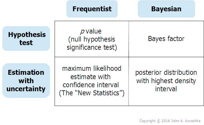
The image below contrasts the tools used for estimation and hypothesis testing in Bayesian and frequentist statistics. For now, focus on the Bayesian column.
To learn more about how this works, let's turn back to Bayes Rules!.
Chapter 8 Posterior Inference & Prediction
This section explains how to use the posterior distribution to test a hypothesis, introducing concepts like posterior probability and the Bayes Factor.
Read the section '8.2 Posterior hypothesis testing.' Focus on the logic: we start with prior odds, collect data, and end up with posterior odds. The Bayes Factor is the engine that drives this change.
Test your understanding!
For each scenario below, decide whether the primary goal is estimation or hypothesis testing.
- An e-commerce company has run an A/B test on a new "checkout" button. They want to determine if the new button (B) has a higher click-through rate than the old one (A).
- A climate scientist has a model that predicts average global temperature rise. They want to provide a range of likely temperature increases by the year 2050.
- You're analyzing user engagement for your app. You want to determine the average number of sessions per user per week and communicate your uncertainty about this number.
Show answer
- Hypothesis Testing. The core question is a comparison between two competing claims: : "The new button is not better" vs. : "The new button is better".
- Estimation. The goal is to determine a value (the temperature increase) and quantify the uncertainty around it by providing a range of plausible values (a credible interval).
- Estimation. Similar to the previous example, the goal is to find a plausible range for an unknown parameter (average sessions per user).
3. Goal 3: Prediction (What will happen next?)
The final major goal is prediction. After observing some data and updating our beliefs about a parameter, we can use that knowledge to predict future, unseen data.
A key strength of the Bayesian approach is that predictions naturally incorporate our uncertainty. A Bayesian prediction isn't a single number; it's a full probability distribution called the posterior predictive distribution. This distribution accounts for two sources of uncertainty:
- Posterior Uncertainty: Our uncertainty about the true value of the parameter (e.g., we don't know the exact bias of the coin).
- Sampling Uncertainty: The inherent randomness in the data-generating process (e.g., even with a fair coin, we don't know if the next flip will be heads or tails).
This produces more realistic and honest forecasts. Instead of predicting that "we will sell 105 units next month," a Bayesian model might say "we will most likely sell between 80 and 130 units, with the peak of the probability distribution around 105."
The final reading selection explains this concept clearly.
Chapter 8 Posterior Inference & Prediction
This last section introduces the concept of the posterior predictive distribution, explaining how it combines two different sources of variability to make robust predictions.
Read the section '8.3 Posterior prediction.' Focus on understanding the two sources of variability (sampling and posterior) that are combined to create a posterior predictive model.
Conclusion
Today, we've mapped out the three main things you can do once you have a posterior distribution. All of the practical Bayesian modeling you'll do in the future will be in service of one or more of these goals.
Key Takeaways:
- Estimation is about summarizing the plausible values of an unknown parameter, typically using a credible interval to express uncertainty.
- Hypothesis Testing is about comparing the relative plausibility of competing claims, often using the Bayes factor to quantify the strength of evidence.
- Prediction is about forecasting future data, using the posterior predictive distribution which incorporates uncertainty about both the parameters and the data itself.
- A powerful feature of Bayesian inference is that all three of these tasks flow naturally from a single source: the posterior distribution.
Next time:
We've established the "what" and "why" of Bayesian analysis. Now it's time to get our hands dirty with the "how." In the next lesson, we will begin Module 2 and learn the mechanics of performing a Bayesian update for problems with discrete hypotheses using a simple, table-based method. This will be our first step towards performing these three tasks in practice.