Missing Data: Imputation and Removal

1. The Nature of Missing Data

Before we jump into the code, it's important to understand why data might be missing. The reason can influence which strategy you choose.

In short:

• Missing Completely at Random (MCAR): The missingness is random and has no connection to any other data. This is the ideal scenario.
• Missing at Random (MAR): The missingness is related to another variable in the dataset, but not the missing value itself.
• Missing Not at Random (MNAR): The missingness is related to the value that is missing. This is the trickiest to handle as it can introduce significant bias.

This flowchart provides a great mental model for the process we'll follow today, from identification to choosing a solution.

2. Finding the Gaps: Identifying Missing Data

Your first step is always to identify where and how much data is missing. Pandas gives you simple and effective tools for this.

To summarize, df.info() gives you a count of non-null values, while df.isna().sum() (or its alias df.isnull().sum()) gives you a direct count of null (NaN) values for each column. The latter is typically the most direct way to assess the extent of the problem.

3. Strategy 1: Removal (Dropping Data)

The simplest strategy is to remove the rows or columns that contain missing data. This is often a good choice if the amount of missing data is very small and randomly distributed (MCAR), as the loss of information will be minimal.

Dropping Rows

By default, .dropna() removes any row containing at least one NaN value.

Dropping Columns

You can also remove entire columns if they are not critical to your analysis and contain a large number of missing values. You do this with the axis=1 parameter.

Another very useful parameter is thresh, which lets you specify the minimum number of non-missing values a row must have to be kept.

Pros and Cons of Removal

• Pro: Simple and effective if the proportion of missing data is small.
• Con: Can lead to significant information loss if many rows are dropped, potentially introducing bias into your dataset.

import pandas as pd
import numpy as np

df = pd.DataFrame({
    'A': [1, 2, np.nan, 4],
    'B': [5, np.nan, 7, 8],
    'C': [9, 10, 11, np.nan],
    'D': [np.nan, np.nan, np.nan, np.nan]
})

4. Strategy 2: Imputation (Filling Data)

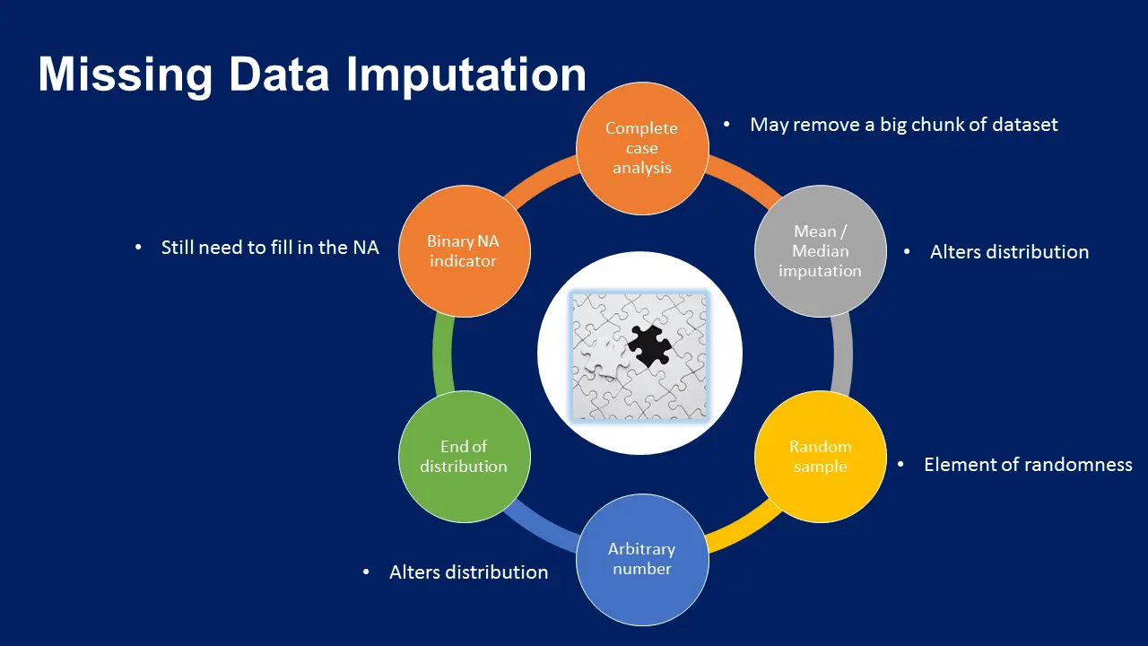
Instead of deleting data, we can fill in the blanks. This is called imputation. The challenge is to fill the missing values with reasonable estimates without distorting the data's original distribution.

Simple Imputation Methods

These are straightforward and widely used for their simplicity. The main function is .fillna().

1. Filling with a Constant: You can replace NaN with 0 for numerical data or a string like "Unknown" for categorical data. This is useful when the absence of a value is meaningful in itself.
2. Filling with a Statistic (Mean/Median/Mode):
   • Mean: Good for numerical columns that are roughly normally distributed. Sensitive to outliers.
   • Median: Better for numerical columns with outliers or a skewed distribution.
   • Mode: Used for categorical (string) columns.
3. Forward Fill and Backward Fill (ffill, bfill): This propagates the last valid observation forward or the next valid observation backward. It's especially useful for time-series data where values are likely to be similar to the preceding or following ones.

Advanced Imputation: Interpolation

Interpolation is a more sophisticated way to estimate missing values, particularly for numerical or time-series data. Instead of just copying a value, it estimates a value that lies between other data points. Linear interpolation, for example, draws a straight line between the points before and after the gap and picks the value on that line.

Your CS and math background will help you appreciate this. It's like finding a point on a line given two other points—a more "intelligent" guess than just taking the average of the whole dataset.

Assessing the Impact of Imputation

Crucially, you must be aware that imputation changes your data. A good imputation strategy preserves the original statistical distribution of the data as much as possible. A poor one can distort it.

This visual check is a powerful tool to validate your imputation strategy. If the shape of your data's distribution changes drastically after filling in values, you may be introducing significant bias.

Conclusion

You have now learned the essential strategies for handling missing data in Pandas, a critical skill for any data scientist or machine learning practitioner.

Key Takeaways:

• Identify First: Always start by using .isna().sum() to understand the scope of your missing data problem.
• Removal (.dropna()): A simple and fast method, but best used when the amount of missing data is small to avoid significant information loss.
• Imputation (.fillna(), .interpolate()): A more common approach where you fill in missing values. The choice of method is critical:
  • Mean/Median/Mode: Simple statistical fills. Use Median if outliers are present.
  • Forward/Backward Fill: Excellent for ordered or time-series data.
  • Interpolation: A more sophisticated guess for numerical data that often yields better results.
• No Perfect Solution: Every method has trade-offs. The goal is to choose the one that makes the most sense for your specific data and problem, and which introduces the least amount of distortion.

Preview of the Next Lesson:
This lesson marks the end of our core Pandas module. You've built a strong foundation in loading, inspecting, filtering, sorting, transforming, and now cleaning data. In our next module, "Data Visualization and Preparation," we will begin to explore our data visually. Our first lesson will focus on creating basic plots like line charts, scatter plots, and histograms using Matplotlib, allowing you to see the patterns and distributions in the data you've worked so hard to prepare.