Data Transformation: Functions & New Columns

1. The Fastest Way: Vectorized Operations

Before reaching for more complex functions, you should always see if you can accomplish your goal with direct, or "vectorized," operations. Since your background is in computer science, you can think of this as similar to how NumPy leverages low-level, compiled code (C or Fortran) to perform operations on entire arrays at once, rather than iterating in Python. Pandas is built on NumPy and inherits this power.

If you want to create a new column by performing a simple arithmetic operation on other columns, this is the best and most efficient approach.

Let's solidify this with an example. Imagine a DataFrame grades:

import pandas as pd

grades_df = pd.DataFrame({
    'student': ['Alice', 'Bob', 'Charlie'],
    'midterm_score': [85, 91, 78],
    'final_score': [92, 88, 81]
})

To create a total_score column, you don't need a loop or a special function. You can just write:

grades_df['total_score'] = grades_df['midterm_score'] + grades_df['final_score']
print(grades_df)

Output:

   student  midterm_score  final_score  total_score
0    Alice             85           92          177
1      Bob             91           88          179
2  Charlie             78           81          159

This is clean, readable, and performs extremely well. Always try this first.

2. Transforming a Single Column: .map() and .apply()

What if your transformation isn't a simple arithmetic operation? For transformations on a single column (a Pandas Series), you have two main tools: .map() and .apply().

Using .map() for Value Substitution

The .map() method is perfect for substituting each value in a column with another value. It's most powerful when you provide a dictionary for the mapping. This is extremely common in machine learning for encoding categorical variables into numbers.

As you saw, .map() is ideal for this kind of direct replacement. While you could achieve this with .apply(), .map() is significantly faster for this specific task.

Using .apply() for Custom Functions on a Series

When your transformation on a single column is more complex than a simple dictionary mapping, Series.apply() is your tool of choice. It takes a function (which can be a lambda function) and applies it to each element in the column.

3. Creating New Columns from Multiple Columns: DataFrame.apply()

This is where the real power of .apply() on a DataFrame comes in. When you need to create a new column whose value depends on complex logic involving multiple other columns in the same row, and this logic can't be easily vectorized, DataFrame.apply() with axis=1 is the way to go.

When you use .apply(axis=1), Pandas iterates through each row of the DataFrame and passes the row (as a Series object) to your custom function. Your function can then access the values of that row using column names, perform its logic, and return a single value for the new column.

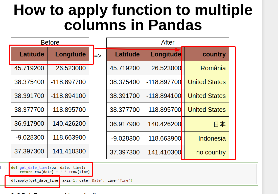
Let's see a concrete example.

A Word on Performance: While incredibly flexible, DataFrame.apply(axis=1) is essentially a loop at the Python level. It can be slow on very large datasets. That's why it's important to always prefer vectorized operations when possible. Use .apply(axis=1) when your logic is too complex to be vectorized.

grades_df = pd.DataFrame({
    'student': ['Alice', 'Bob', 'Charlie'],
    'midterm_score': [85, 91, 78],
    'final_score': [92, 88, 81]
})

grades_df['passed'] = grades_df.apply(lambda row: row['final_score'] > 85, axis=1)
print(grades_df)

   student  midterm_score  final_score  passed
0    Alice             85           92    True
1      Bob             91           88    True
2  Charlie             78           81   False

4. Advanced Topic: Returning Multiple Columns from apply

What if your function calculates several new values at once? Instead of running .apply() multiple times, you can write a function that returns a list or a Pandas Series. This is a more advanced pattern but is very efficient from a coding perspective.

5. Quick Mention: .applymap()

For completeness, there is one other method, .applymap(). It is used to apply a function to every single element in an entire DataFrame. Its use cases are less common, but you might use it to, for example, format all numbers in a table to a certain number of decimal places if all columns were numeric.

Think of it this way:

• .map(): Element-wise on a Series.
• .applymap(): Element-wise on a DataFrame.
• .apply(): Row/column-wise on a DataFrame or element-wise on a Series.

Conclusion

You've now learned the primary methods for transforming data and creating new columns in Pandas. This is a huge step towards preparing data for analysis and machine learning.

Key Takeaways:

• Vectorized Operations: Always your first choice for speed and simplicity (e.g., df['C'] = df['A'] + df['B']).
• Series.map(): The best tool for substituting values in a single column, especially with a dictionary. It's fast and purpose-built for this task.
• Series.apply(): Use this to apply a custom function to each element of a single column when a dictionary mapping isn't sufficient.
• DataFrame.apply(axis=1): Your powerful, flexible tool for creating new columns when the logic requires values from multiple columns in the same row. Use it when vectorization isn't possible.
• Performance Matters: Remember the general hierarchy from fastest to slowest: Vectorized operations > .map() > .apply().

Preview of the Next Lesson:
Transforming data can sometimes introduce or reveal missing values (NaN). In our next lesson, we'll tackle this head-on by learning how to handle missing data using various strategies like removal and imputation. This is another non-negotiable step in building robust data pipelines.